
Market Microstructure in MQL5 (Part 7): Regime Classification

Introduction
Part 1 built the defensive foundation. Parts 2 and 3 measured whether price has memory. Part 4 measured what volatility is doing and whether it persists. Part 5 decomposed price variation into noise and signal. Part 6 measured the direction of informed flow. Parts 2-6 together produce eleven distinct measurements of the market environment on the one-minute timeframe.
Each measurement is individually informative. Together they are correlated, partially redundant, and impossible to act on simultaneously in real time. A position-sizing system cannot respond to eleven separate signals. What is needed is a reduction: a single composite label that summarises the current session environment, and a confidence score that reflects how reliably the available measurements agree.
Part 7 implements this reduction. RegimeClassifier() takes the outputs of Parts 2-6 and assigns one of six regime labels (Normal, Stressed, Noisy, Informed, Trending, Mean-Reverting). It also returns a confidence score in [0, 1] and a composite directional score in [-1, +1]. The classification boundaries are derived empirically from 514 NQ M1 sessions, and the six labels correspond to distinct trading environments that warrant different responses in position sizing, stop placement, and signal filtering.
The classifier uses a priority-ordered rule set rather than a statistical model. This is a deliberate design choice. A machine learning classifier (k-means, random forest, hidden Markov model) would require out-of-sample validation, which is not feasible within a single article. A rule-based classifier is fully transparent, directly connected to the empirical thresholds derived in Parts 4-6, and immediately actionable without a training step. The rules are documented in full, and readers are encouraged to recalibrate the thresholds on their own instruments and sample periods.
Deliverable: one classification function, a MARKET_REGIME enumeration, a new RegimeAnalysis struct, and PopulateRegimeAnalysis() that calls the full measurement chain from Parts 2-6 in sequence. No new include file is created. The companion SSRN paper is at SSRN 6847024.
The Six Regimes
Normal Normal is the residual - sessions that do not meet the threshold for any of the five named regimes. It accounts for 50% of sessions in the NQ M1 empirical study. Normal sessions have near-mean noise (0.585), clustering (0.142), and flow confidence (0.722). The composite directional score is near zero (0.036) - there is no reliable directional signal. Standard realized volatility and position sizing based on the Part 4 thresholds apply directly.
StressedStressed sessions are identified by one or more of: flow_confidence equal to zero (jump-contaminated session from Part 4), realized vol above the 90th percentile, or the combination of vol above the 75th percentile and noise above the 75th percentile simultaneously. Stressed sessions account for 21% of the sample. They have 1.8x normal realized volatility and substantially lower flow confidence (0.430 vs 0.722 for Normal). The composite score is zero - the regime carries no directional signal. Reduce position size materially or stand aside.
NoisyNoisy sessions have noise ratio above the 75th percentile (0.632) and flow confidence below the 25th percentile (0.679). These are sessions where more than the typical fraction of price variation is transient friction and the order flow signal is specifically flagged as unreliable. They account for 10% of the sample. Mean noise ratio is 0.674 - among the highest of any regime. Clustering is 0.102, well below the Normal mean of 0.142, meaning that not only is noise high but vol predictability is also low. Widen stops and discount the Part 4 clustering signal.
InformedInformed sessions require all four conditions simultaneously: VPIN above the 75th percentile (0.539), noise below the 75th percentile, clustering above the median (0.138), and flow confidence above the 25th percentile. This conjunction ensures the elevated volume imbalance is occurring in a clean signal environment rather than a noisy one. Informed sessions account for 7% of the sample. They have the highest VPIN (0.559), elevated clustering (0.231), and a positive composite score (0.270) - all consistent with directional informed activity. Align position with the flow imbalance direction and use tighter stops.
TrendingTrending sessions require clustering above the 75th percentile (0.203) and multifractal width below the median (0.875), with noise below the 75th percentile. High clustering means volatility is predictable bar-to-bar. A low multifractal width means the session's scaling is closer to monofractal - the price process is dominated by a single Hurst exponent rather than a mixture of opposing memory regimes. This combination is consistent with a session where directional momentum is structurally present and the Part 4 volatility measures can be trusted. Trending sessions have the highest clustering of any regime (0.286, 2x Normal), the highest composite score (0.356), and the highest mean confidence (0.593). These are the sessions where momentum strategies have the strongest theoretical support.
Mean-RevertingMean-Reverting sessions require the ARFIMA d estimate below the 25th percentile (-0.061) and clustering below the 25th percentile (0.076). Strongly negative d and low clustering indicate anti-persistent returns. In such sessions, reversals are stronger than a random walk implies, and squared-return autocorrelation provides no bar-to-bar predictability. Mean-Reverting sessions have the lowest clustering of any regime (0.032) and a negative composite score (-0.202), which means fading the directional flow is the indicated strategy. They account for 4% of the sample - the rarest named regime.
Classification Logic
Priority ordering The classifier applies six rules in priority order. The first matching rule determines the regime; subsequent rules are not evaluated. Priority order is:
- Stressed - checked first because elevated risk overrides all other signals
- Informed - elevated volume imbalance in a clean environment
- Trending - high clustering and monofractal structure
- Noisy - elevated noise with low flow confidence
- Mean-Reverting - strongly negative d with low clustering
- Normal - residual
The ordering is a design choice, not a statistical optimum. The choice to evaluate Stressed before Informed prevents a jump-contaminated session with elevated VPIN from being misclassified as Informed. The choice to evaluate Trending before Noisy prevents a high-clustering session that also has elevated noise from being masked by the noise label.
Confidence scoreThe confidence score combines the rule-match score with a reliability multiplier based on measurement quality. The reliability multiplier is the geometric mean of the MFDFA R-squared confidence from Part 3 and the flow_confidence from Part 6. Roll confidence is excluded from the reliability calculation - as documented in Part 5, it is near-zero on NQ M1 and would suppress all confidence scores if included. This is a direct consequence of the M1 aggregation limitation documented across Parts 5 and 6.
Composite directional scoreThe composite score is a signed directional signal in [-1, +1]. For Trending and Informed sessions, the sign follows the flow imbalance direction and the magnitude reflects the confidence. For Mean-Reverting sessions, the sign is the opposite of the flow imbalance - fade the current direction. For Stressed and Noisy sessions, the composite score is zero - no directional signal is offered when the environment is adverse. For Normal sessions, the composite score is a weak positive signal scaled by flow confidence.
Implementation
MARKET_REGIME enumeration and RegimeAnalysis struct //+------------------------------------------------------------------+ //| MARKET_REGIME: six-state regime classification. | //| Used in RegimeAnalysis.regime field. | //+------------------------------------------------------------------+ enum MARKET_REGIME { REGIME_NORMAL = 0, // Residual - no named regime applies REGIME_STRESSED = 1, // Elevated vol/noise/jumps - reduce size REGIME_NOISY = 2, // High noise + low flow confidence REGIME_INFORMED = 3, // Elevated VPIN in clean environment REGIME_TRENDING = 4, // High clustering + monofractal structure REGIME_MEAN_REVERTING = 5, // Anti-persistent d + low clustering }; //+------------------------------------------------------------------+ //| RegimeAnalysis: composite regime classification result. | //| Populated by RegimeClassifier() or PopulateRegimeAnalysis(). | //| composite_score: signed directional signal [-1,+1]. | //| Trending/Informed: follow flow direction. | //| Mean-Reverting: fade flow direction. | //| Stressed/Noisy: zero - no directional signal. | //+------------------------------------------------------------------+ struct RegimeAnalysis { MARKET_REGIME regime; // Current regime label double confidence; // Classification confidence [0,1] double composite_score; // Signed directional score [-1,+1] };RegimeClassifier()
The classifier accepts the populated structs from Parts 3-6 by const reference and returns a RegimeAnalysis. All threshold constants are defined at the top of the function for easy recalibration. The reliability multiplier uses the geometric mean of MFDFA R-squared confidence and flow_confidence only - roll confidence is excluded as documented in Part 5.
//+------------------------------------------------------------------+
//| RegimeClassifier: priority-ordered rule-based regime classifier. |
//|                                                                  |
//| Thresholds calibrated from 514 NQ M1 sessions (May 2024 -        |
//| May 2026). Recalibrate on your own instrument and sample period. |
//|                                                                  |
//| Priority (first match wins):                                     |
//|   1. STRESSED      - vol/noise/jump threshold exceeded           |
//|   2. INFORMED      - VPIN + clustering + low noise (all four)    |
//|   3. TRENDING      - clustering P75 + delta_alpha < median    |
//|   4. NOISY         - noise P75 + flow_confidence P25             |
//|   5. MEAN_REVERTING- GPH d P25 + clustering P25                  |
//|   6. NORMAL        - residual                                    |
//+------------------------------------------------------------------+
RegimeAnalysis RegimeClassifier(const RobustFractalAnalysis  &rfa,
                                 const VolatilityAnalysis     &va,
                                 const MicrostructureAnalysis &msa,
                                 const OrderFlowAnalysis      &ofa)
  {
   RegimeAnalysis result;
   result.regime          = REGIME_NORMAL;
   result.confidence      = 0.0;
   result.composite_score = 0.0;

   //--- Thresholds (NQ M1, May 2024-May 2026 calibration)
   const double RV_P75      = 0.000501; // realized_vol 75th pct
   const double RV_P90      = 0.000630; // realized_vol 90th pct
   const double NOISE_P75   = 0.6317;   // noise_ratio 75th pct
   const double NOISE_P25   = 0.5666;   // noise_ratio 25th pct
   const double VPIN_P75    = 0.5393;   // vpin 75th pct
   const double CL_P75      = 0.2026;   // clustering_idx 75th pct
   const double CL_P25      = 0.0756;   // clustering_idx 25th pct
   const double CL_MED      = 0.1376;   // clustering_idx median
   const double DA_MED      = 0.8747;   // delta_alpha median
   const double GPH_P25     = -0.0611;  // gph_d 25th pct
   const double FC_P25      = 0.6790;   // flow_confidence 25th pct

   //--- Input fields
   double rv     = va.realized_vol;
   double noise  = msa.noise_ratio;
   double vpin   = ofa.vpin;
   double cl     = va.clustering_index;
   double da     = rfa.multifractal_width;
   double gph_d  = rfa.arfima_d;
   double fc     = ofa.flow_confidence;
   double flow_i = ofa.flow_imbalance;
   double mfdfa_c= rfa.dimension_confidence;

   //--- Reliability: geometric mean of MFDFA confidence and flow confidence
   //--- Roll confidence excluded - near-zero on NQ M1 (Part 5)
   double mfdfa_safe = MathMax(0.01, MathMin(1.0, mfdfa_c));
   double fc_safe    = MathMax(0.05, fc);
   double reliability= MathSqrt(mfdfa_safe * fc_safe);

   //--- 1. STRESSED
   int s_count = 0;
   if(fc <= 0.0)                             s_count++; // jump-contaminated
   if(rv > RV_P90)                            s_count++; // extreme vol
   if(rv > RV_P75 && noise > NOISE_P75)      s_count++; // vol + noise spike
   if(s_count > 0)
     {
      result.regime     = REGIME_STRESSED;
      result.confidence = MathMin(1.0, 0.55 + 0.15*s_count) * reliability;
      return result;  // composite_score = 0 for stressed
     }

   //--- 2. INFORMED: all four conditions required
   if(vpin  > VPIN_P75
      && noise < NOISE_P75
      && cl    > CL_MED
      && fc    > FC_P25)
     {
      double conf = MathMin(1.0,
                    0.55 + (vpin - VPIN_P75) * 5.0) * reliability;
      result.regime          = REGIME_INFORMED;
      result.confidence      = conf;
      result.composite_score = MathSign(flow_i) * conf * 0.5;
      return result;
     }

   //--- 3. TRENDING: clustering P75 + delta_alpha below median
   if(cl    > CL_P75
      && da    < DA_MED
      && noise < NOISE_P75)
     {
      double conf = MathMin(1.0,
                    0.50 + (cl - CL_P75) / 0.40) * reliability;
      result.regime          = REGIME_TRENDING;
      result.confidence      = conf;
      result.composite_score = MathSign(flow_i) * conf * 0.6;
      return result;
     }

   //--- 4. NOISY: noise P75 + flow_confidence P25
   if(noise > NOISE_P75 && fc < FC_P25)
     {
      double conf = MathMin(1.0,
                    0.50 + (noise - NOISE_P75) * 3.0) * reliability;
      result.regime     = REGIME_NOISY;
      result.confidence = conf;
      return result;  // composite_score = 0 for noisy
     }

   //--- 5. MEAN-REVERTING: GPH d P25 + clustering P25
   if(gph_d < GPH_P25 && cl < CL_P25)
     {
      double conf = MathMin(1.0,
                    0.45 + MathAbs(gph_d) * 1.5) * reliability;
      result.regime          = REGIME_MEAN_REVERTING;
      result.confidence      = conf;
      result.composite_score = -MathSign(flow_i) * conf * 0.4;
      return result;
     }

   //--- 6. NORMAL: residual
   result.regime          = REGIME_NORMAL;
   result.confidence      = MathMin(1.0,
                             0.30 + 0.40*fc) * reliability;
   result.composite_score = 0.05 * MathSign(flow_i) * fc;
   return result;
  }
PopulateRegimeAnalysis()
The full measurement chain wrapper calls all six Populate() functions in sequence and then runs the classifier. This is the single entry point for users who want the complete chain in one call. An overload that accepts pre-populated structs is also provided for users who call individual Populate() functions separately.
//+------------------------------------------------------------------+
//| PopulateRegimeAnalysis: full measurement chain + classifier.     |
//| Calls Parts 2-6 Populate() functions in sequence.                |
//| vol_baseline: 20-session rolling mean bar volume (caller).       |
//+------------------------------------------------------------------+
void PopulateRegimeAnalysis(const string symbol, const int tf,
                             const int period,
                             RegimeAnalysis         &regime_out,
                             RobustFractalAnalysis  &rfa,
                             VolatilityAnalysis     &va,
                             MicrostructureAnalysis &msa,
                             OrderFlowAnalysis      &ofa,
                             double vol_baseline = 0.0)
  {
   PopulateHurstAnalysis          (symbol, tf, period, rfa);
   PopulateMultifractalAnalysis   (symbol, tf, period, rfa);
   PopulateVolatilityAnalysis     (symbol, tf, period, va, rfa);
   PopulateMicrostructureAnalysis (symbol, tf, period, msa, rfa);
   PopulateOrderFlowAnalysis      (symbol, tf, period, ofa, msa, va,
                                   vol_baseline);
   regime_out = RegimeClassifier  (rfa, va, msa, ofa);
  }

//+------------------------------------------------------------------+
//| Overload: classifier only (pre-populated structs).               |
//+------------------------------------------------------------------+
void PopulateRegimeAnalysis(const RobustFractalAnalysis  &rfa,
                             const VolatilityAnalysis     &va,
                             const MicrostructureAnalysis &msa,
                             const OrderFlowAnalysis      &ofa,
                             RegimeAnalysis               &regime_out)
  {
   regime_out = RegimeClassifier(rfa, va, msa, ofa);
  }
Empirical Study: NQ M1 Regime Classification
The classifier was applied to 514 NY sessions of NQ M1 futures (May 2024-May 2026) using the merged outputs of Parts 4, 5, and 6. The thresholds used are those calibrated from this dataset and shown in the classifier function above. All four named stress episodes from Parts 4-6 are present in the sample.
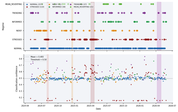
Figure 1 - Top: regime classification across 514 NQ sessions (May 2024-May 2026). Each dot is one session; dot size reflects classification confidence. Bottom: confidence time series colored by regime. The April 2025 tariff shock and BoJ shock are classified entirely as STRESSED. The April 2026 tariff episode is predominantly NORMAL.
Table 1 - Regime Frequency (514 sessions, NQ M1)| Regime | Sessions | % | Mean confidence | Mean composite score |
|---|---|---|---|---|
| Normal | 257 | 50.0% | 0.493 | 0.036 |
| Stressed | 110 | 21.4% | 0.444 | 0.000 |
| Noisy | 51 | 9.9% | 0.484 | 0.000 |
| Informed | 38 | 7.4% | 0.540 | 0.270 |
| Trending | 37 | 7.2% | 0.593 | 0.356 |
| Mean-Reverting | 21 | 4.1% | 0.505 | -0.202 |
The distribution is well-balanced: no regime is empty and the Normal residual at 50% is consistent with a market that spends roughly half its time in an undifferentiated state. The Trending and Mean-Reverting regimes at 7% and 4% respectively reflect their definition - they require multiple conditions to fire simultaneously, which is deliberately restrictive. The Stressed regime frequency (21%) is higher than expected. This reflects the NQ M1 sample period, which includes four identifiable macro events and generally elevated volatility from April 2025 onward.
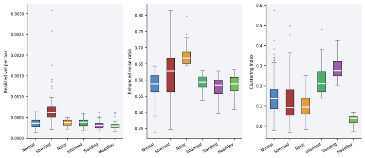
Figure 2 - Realized vol (left), noise ratio (center), and clustering index (right) by regime. The internal consistency check: Trending has the highest clustering, Mean-Reverting the lowest. Noisy has the highest noise ratio. Stressed has the widest vol distribution. These separations confirm the classifier is capturing distinct market environments rather than arbitrary partitions.
Table 2 - Regime Characteristics| Regime | Realized vol | vs Normal | Noise ratio | Clustering | Flow conf | VPIN-60 |
|---|---|---|---|---|---|---|
| Normal | 0.000364 | - | 0.585 | 0.142 | 0.722 | 0.514 |
| Stressed | 0.000671 | 1.8x | 0.620 | 0.123 | 0.430 | 0.533 |
| Noisy | 0.000393 | 1.1x | 0.674 | 0.102 | 0.621 | 0.543 |
| Informed | 0.000395 | 1.1x | 0.594 | 0.231 | 0.718 | 0.559 |
| Trending | 0.000348 | 0.96x | 0.578 | 0.286 | 0.726 | 0.514 |
| Mean-Reverting | 0.000311 | 0.85x | 0.585 | 0.032 | 0.722 | 0.519 |
The internal consistency of the classifier is visible in the characteristics table. Trending has the highest clustering (0.286, 2.0x Normal) by construction - clustering above the 75th percentile is a required condition. Mean-Reverting has the lowest clustering (0.032) by construction - clustering below the 25th percentile is required. Noisy has the highest noise ratio (0.674) by construction. These are not coincidences; they confirm the classifier conditions are correctly implemented.
Three findings go beyond the mechanical. Stressed sessions have meaningfully lower flow confidence (0.430 vs 0.722) despite not explicitly requiring this - the jump contamination condition and the vol threshold together capture sessions where the order flow signal deteriorates. Informed sessions have the highest VPIN (0.559) without this being a sufficient condition on its own - the conjunction requirement filters out high-VPIN sessions that occur in noisy environments. Trending sessions have below-normal realized vol (0.96x Normal) - a consistent finding that directional momentum is associated with orderly rather than turbulent price action.
Stress episode alignmentThe classifier assigns regimes to the four named stress episodes as follows:
| Episode | Sessions | STRESSED | Other | Interpretation |
|---|---|---|---|---|
| BoJ shock (Aug 2024) | 8 | 8 (100%) | 0 | Pure vol event - all sessions captured |
| Tariff Apr 2025 | 14 | 14 (100%) | 0 | Highest-vol episode - all captured |
| Fed Dec (Dec 2024) | 6 | 3 (50%) | 3 (Informed/Normal) | Moderate event - partial capture |
| Tariff Apr 2026 | 18 | 1 (6%) | 17 (Normal/Trending) | Adaptation - market not stressed |
The BoJ and April 2025 episodes are captured entirely as Stressed, consistent with their extreme vol and noise characteristics in Parts 4 and 5. The Fed December 2024 episode is only partially captured. Three of six sessions exceed the vol thresholds. The remaining three sessions are classified as Informed or Normal. This reflects an event that was acute but short-lived, and not uniformly severe across its six-session window.
The April 2026 tariff episode is classified as predominantly Normal (15/18 sessions) with two Trending and one Stressed session. This is the correct result given the empirical data: Part 4 showed below-normal vol (0.91x Normal), Part 5 showed below-normal noise (0.564 vs 0.603 for Normal), and Part 6 showed the highest SMI in the dataset (0.147). The market had adapted. The regime classifier confirms this adaptation without requiring it - the Normal and Trending classifications emerge from the data, not from a special-case rule for the 2026 episode.
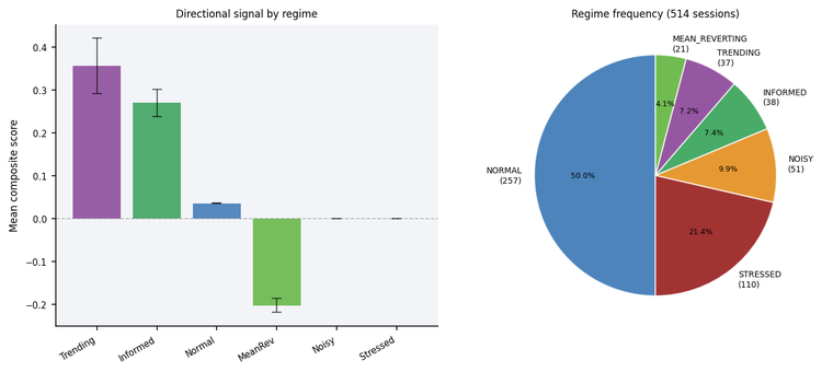
Figure 3 - Left: mean composite directional score by regime with standard deviation bars. Trending (0.356) and Informed (0.270) carry positive directional signals; Mean-Reverting (-0.202) carries a negative signal (fade the current direction). Stressed and Noisy carry no directional signal. Right: regime frequency distribution across 514 sessions.
LimitationsThe regime classifier is a rule-based system calibrated to NQ M1 over a specific 27-month window. Three limitations apply directly.
First, the thresholds are empirical percentile cutoffs from a single instrument and sample period. They are not statistically derived decision boundaries and are not optimal in any formal sense. A different instrument, timeframe, or sample period will have different distributions of vol, noise, clustering, and d - users should re-derive all thresholds on their own data before applying the classifier in production. The threshold constants are grouped at the top of RegimeClassifier() for exactly this reason.
Second, the priority ordering of the rules is a design choice, not an optimum. The ordering places Stressed first and Normal last, which is conservative - it favours caution over signal. A different priority order would produce different regime frequencies. For example, placing Trending above Stressed would reclassify some high-vol, high-clustering sessions as Trending rather than Stressed. Neither ordering is objectively correct; the choice should reflect the risk tolerance of the application.
Third, the classifier is not validated out-of-sample. The thresholds are calibrated and applied to the same 514-session dataset. Out-of-sample validation - testing whether regime labels predict future returns or strategy performance on held-out data - is documented in the companion SSRN paper. The current article delivers the measurement layer only.
The underlying metrics are also limited by M1 aggregation, as documented in Parts 5 and 6. The Roll spread and VPIN_OHLC are approximate at one-minute resolution. The regime classifier inherits these approximations and is correspondingly limited in its ability to detect informed flow at the bar level. Users with tick data should compute the underlying metrics at tick resolution before classifying - the RegimeClassifier() function accepts any pre-populated structs and is agnostic to how they were populated.
Practical UsageThe thresholds in RegimeClassifier() are defined as local constants and should be adjusted for your instrument and timeframe. The workflow for recalibration is: run the Part 4-6 Populate() functions across a historical sample, compute the key percentiles from the output, and replace the constant values.
//--- Full measurement chain: one call from OnTick() or OnBar()
RobustFractalAnalysis  rfa;
VolatilityAnalysis     va;
MicrostructureAnalysis msa;
OrderFlowAnalysis      ofa;
RegimeAnalysis         reg;

PopulateRegimeAnalysis(Symbol(), PERIOD_M1, 390, reg, rfa, va, msa, ofa,
                       vol_baseline);   // vol_baseline: 20-session rolling mean

//--- Regime-conditioned position sizing
double base_size = 1.0;
switch(reg.regime)
  {
   case REGIME_STRESSED:
      base_size = 0.0;   // stand aside
      break;
   case REGIME_NOISY:
      base_size = 0.3;   // reduce materially
      break;
   case REGIME_TRENDING:
      base_size = 1.2;   // increase modestly
      break;
   case REGIME_INFORMED:
      base_size = 1.0;   // normal, but align with composite direction
      break;
   case REGIME_MEAN_REVERTING:
      base_size = 0.7;   // reduce and fade current direction
      break;
   default:              // REGIME_NORMAL
      base_size = 1.0;
      break;
  }

//--- Scale by confidence and composite direction
if(reg.confidence < 0.40) base_size *= 0.5; // low confidence: halve
double direction = (MathAbs(reg.composite_score) > 0.1)
                    ? MathSign(reg.composite_score) : 0.0;
double final_size = direction * base_size * reg.confidence;
Folder Structure and Include Path
All Part 7 additions are made to the existing foundation header. No new files are created. The folder structure remains unchanged:
MQL5\
+-- Indicators\
    +-- HurstProfile\
        +-- HurstProfile.mq5
        +-- Includes\
            +-- MicroStructure_Foundation.mqh
#include "Includes\MicroStructure_Foundation.mqh"
Conclusion
The RegimeClassifier() function reduces the eleven measurements from Parts 2-6 to a single actionable label and confidence score. The six regime categories - Normal, Stressed, Noisy, Informed, Trending, and Mean-Reverting - correspond to distinct market environments with different vol, noise, clustering, and flow characteristics, confirmed by the cross-regime statistics from 514 NQ M1 sessions.
The empirical study produces four findings that extend the series narrative. The BoJ and April 2025 episodes are classified entirely as Stressed - pure vol events that correctly receive zero directional signal. The April 2026 episode is classified as predominantly Normal and Trending - market adaptation confirmed at the regime level without requiring special-case treatment. The Trending regime has the highest confidence (0.593) and the strongest directional composite score (0.356) - these are the sessions where the measurement chain from Parts 2-6 produces the most reliable output. The Mean-Reverting regime, at 4% of sessions, is the rarest named regime and the most clearly defined - sessions with strongly negative d and near-zero clustering represent a genuinely distinct structural state.
The out-of-sample validation of the measurement chain - a position-sizing rule conditioned on regime label versus an unconditional baseline - is documented in the companion SSRN paper. Part 8 builds the micro-trend indicator that puts the regime classifier into production use.
Getting the Source Code via MQL5 Algo Forge
Algo Forge provides Git-based version control in the cloud, so you will always have access to the latest version of the code, including any updates or fixes made after this article was published. The full repository is available at MQL5 Algo Forge.
References- Brown, Max (2026). Intraday Microstructure Dynamics of E-mini S&P 500 Futures (May 29, 2026). Available at SSRN: https://ssrn.com/abstract=6847024.
- Hamilton, J.D. (1989). A new approach to the economic analysis of nonstationary time series and the business cycle. Econometrica, 57(2), 357-384.
- Easley, D., Lopez de Prado, M.M. & O'Hara, M. (2012). Flow toxicity and liquidity in a high-frequency world. Review of Financial Studies, 25(5), 1457-1493.
- Lopez de Prado, M.M. (2018). Advances in Financial Machine Learning. Wiley.
- Previous publications
Warning: All rights to these materials are reserved by MetaQuotes Ltd. Copying or reprinting of these materials in whole or in part is prohibited.
This article was written by a user of the site and reflects their personal views. MetaQuotes Ltd is not responsible for the accuracy of the information presented, nor for any consequences resulting from the use of the solutions, strategies or recommendations described.

- Free trading apps
- Over 8,000 signals for copying
- Economic news for exploring financial markets
You agree to website policy and terms of use