Symbolic Aggregate Approximation (SAX) in MQL5: Historical Analog Search and Forecasting

Introduction

Every chart you have ever looked at is a stream of numbers, and almost every tool we build to read it stays in the world of numbers: moving averages, oscillators, regressions, neural networks. There is an older, quieter idea from the time-series mining literature that does something different. It stops treating them as numbers. It takes a window of price, and turns it into a short string of letters, something like bddcbbba. Once a piece of the market is a word, you can do to it everything computer science already knows how to do with text: match it, count it, hash it, search it. That transformation is called Symbolic Aggregate approXimation, or SAX, introduced by Jessica Lin, Eamonn Keogh and colleagues in 2003; their original SAX page collects the papers and is well worth reading.

SAX has been used for fast similarity search, motif discovery, anomaly detection and classification across many scientific fields. In finance it is far less common, and there is an honest reason for that which we will confront head-on rather than hide: the very step that makes SAX elegant, its normalization of each window so only its shape matters, deliberately discards the price level and the volatility, and in trading those are often exactly the information you care about. A method designed to treat any signal alike does not automatically respect what makes a market a market.

This article is not a sales pitch for a magic indicator; it has two goals. First, it implements SAX in pure MQL5, including the Gaussian breakpoints and the lower-bounding distance used for sound search. These primitives are not yet available on the platform. Second, it applies SAX to a practical question: the market is doing this now; when has it behaved similarly before, and what followed? We answer that with an analog-search tool that draws a forecast cone into the future and a verdict panel that reports the statistics behind it. The tool is designed to avoid overclaiming: it withholds forecasts in coin-flip cases, measures outcomes in a volatility-robust way, and prevents any future leakage into the precedent set.

By the end you will have a reusable SAX library, a validation harness that proves the math, and a working indicator, together with a clear understanding of where this technique earns its keep and where it does not.

We will cover:

1. Why Symbolize Price, and the Gap SAX Fills
2. Building the SAX Transform
3. From Words to Precedents: the Analog Search
4. Proving It Works: the Validation Harness
5. The Indicator: Fan Cone and Verdict Panel
6. Conclusion

Why Symbolize Price, and the Gap SAX Fills

Consider the problem SAX was designed to solve. You have a long time series and you want to find repeated shapes in it, or to search for the historical pieces that most resemble a query. Working directly on the raw numbers has two costs that grow with the data. The first is that the space of possible windows is continuous and effectively infinite, so you can never simply count how often a given shape occurs, build a histogram of shapes, or reason about their frequencies. The second is scale: comparing a query against every window in a long history means an enormous number of full distance computations, and there is no cheap way to rule candidates out in advance. SAX attacks both by compressing each window into a few letters drawn from a tiny alphabet. A window becomes one of a finite, countable set of words, the cheap word distance can rule most candidates out before any full comparison, and the reduction smooths away noise along the way.

The transform has three steps, and each one exists for a reason.

Step one: z-normalize the window

We subtract the window's mean and divide by its standard deviation. After this, the window has mean zero and unit standard deviation, so what remains is pure shape. A rise from 1.0800 to 1.0900 on EURUSD and a rise from 2000 to 2020 on gold can map to the same normalized curve if they rise in the same way. This is the source of SAX's power and, in finance, the source of its danger. It is powerful because it lets precedents from different price regimes be compared. It is dangerous because it erases the absolute move and the volatility, and a trader usually needs to know whether a shape played out in a sleepy range or a violent expansion. We do not pretend this away. We compensate for it later, when we measure outcomes, by expressing every forward move in units of the volatility that prevailed at the time.

Step two: Piecewise Aggregate Approximation, the "Aggregate" in SAX

We chop the normalized window into w equal segments and replace each segment with its average. A 48-bar window with w = 8 becomes eight numbers. This is dimensionality reduction, and it is what earns the word "aggregate": it trades away fine detail for a compact, noise-resistant summary of the window's overall trajectory.

Step three: discretize the PAA values into letters

Because the window was z-normalized, its values are approximately standard-normal. So we slice the standard normal distribution into a regions of equal probability using a - 1 breakpoints, and assign each PAA cell the letter of the region it falls in. With a = 4, each of the four letters occurs about a quarter of the time by construction, which keeps the alphabet balanced rather than letting one symbol dominate. Eight cells and four symbols give a word like bddcbbba, and there are only 4^8 = 65,536 possible such words. The infinite space of price windows has become a finite dictionary.

Fig. 1. The SAX transform: a raw price window is z-normalized, reduced by PAA into cells, then each cell is mapped through Gaussian breakpoints to a letter

Two properties lift SAX above a mere gimmick, and both matter to what we build. The first is the lower-bounding distance. SAX defines a distance between two words, called MINDIST, that provably never exceeds the true Euclidean distance between the two underlying normalized series. That guarantee is what makes large-scale search sound: if a cheap word comparison already puts two windows far apart, they are genuinely far apart, so we can discard candidates without risk of throwing away a real match. The second property is simply countability. Because words are finite, you can build histograms of them, count transitions between them, feed them into a Markov model, or treat a collection of windows as a bag of words, all things that are impossible on the raw continuous series.

Now, where does this sit on MQL5 today? A survey of the published catalog shows that the raw ingredients of SAX are absent. There is fine work on alternative representations of time series, for instance the piecewise linear representation used to feed neural networks, and there is a thoughtful recent series, Encoding Candlestick Patterns (Part 1): An Alphabetical System for Signal Detection, that also maps price action to letters. That candlestick series is the closest neighbor to what we do here, and it deserves acknowledgment, because comparing the two approaches is the clearest way to see what makes SAX different. The candlestick-encoding approach assigns letters by rules on each candle's geometry: body size, direction, wick proportions. SAX assigns letters by where a normalized value falls in a probability distribution. One is a hand-designed taxonomy of candle shapes, and a very readable one; the other is a distribution-driven discretization with a provable distance behind it. The two approaches are complementary. PAA, Gaussian breakpoints, MINDIST, and SAX-based analog search do not appear in the published article catalog. That is the gap this article fills.

Read this before the code. SAX normalizes away price level and volatility, and financial returns are noisy and close to a random walk. Applied naively, SAX often has no predictive edge on price at all. This is not a defect we are hiding until the end; it is the design constraint that shapes every decision that follows. The tool we build is deliberately allowed to answer "there is no edge here," and it will do so often. A version of this tool that always shows a confident forecast would be lying to you.

Building the SAX Transform

The transform lives in SAXTransform.mqh as a single class, CSAXTransform. You configure it once with a word length and an alphabet size, and then reuse it to encode as many windows as you like. The header comment states the contract the rest of the code depends on.

//+------------------------------------------------------------------+
//| Symbolic Aggregate approXimation (SAX) — core transform.         |
//|                                                                  |
//|  A raw window of prices is turned into a short string of letters |
//|  in three steps:                                                 |
//|    1. z-normalize the window          (shape, not price level)   |
//|    2. PAA: average it into 'w' cells  (dimensionality reduction) |
//|    3. map each cell to a letter using equal-probability          |
//|       breakpoints of the standard normal   (discretization)      |
//|                                                                  |
//|  Letters are stored as int codes 0..a-1 (0 = lowest band). The   |
//|  MINDIST routine returns a distance between two words that       |
//|  provably lower-bounds the true Euclidean distance of the        |
//|  z-normalized series — this is what makes SAX search sound.      |
//+------------------------------------------------------------------+

We store letters not as characters but as integer codes from 0 to a - 1, where 0 is the lowest band. That keeps the arithmetic in MINDIST clean, and we only render them as human-readable letters when we need to print a word.

The Gaussian breakpoints

The breakpoints are the a - 1 values that cut the standard normal into a equal-probability bands. Breakpoints are zero-indexed here to match the code: for i = 0..a - 2, breakpoint i is the value below which a fraction (i + 1) / a of the distribution lies. In statistics this is the inverse of the normal cumulative distribution function, also called the probit or quantile function. MQL5 has no built-in probit, so we implement Peter Acklam's well-known rational approximation, which is accurate to roughly one part in a billion, far more than we need to place a handful of cut points.

//+------------------------------------------------------------------+
//| Inverse standard-normal CDF (probit) via Acklam's rational       |
//| approximation. Accurate to ~1e-9 over p in (0,1), which is far   |
//| more than the breakpoints need. Returns the z with P(Z<z)=p.     |
//+------------------------------------------------------------------+
double CSAXTransform::NormInv(double p) const
  {
//--- coefficients for Acklam's algorithm
   static const double a1=-3.969683028665376e+01;
   static const double a2= 2.209460984245205e+02;
   static const double a3=-2.759285104469687e+02;
   static const double a4= 1.383577518672690e+02;
   static const double a5=-3.066479806614716e+01;
   static const double a6= 2.506628277459239e+00;

   static const double b1=-5.447609879822406e+01;
   static const double b2= 1.615858368580409e+02;
   static const double b3=-1.556989798598866e+02;
   static const double b4= 6.680131188771972e+01;
   static const double b5=-1.328068155288572e+01;

   static const double c1=-7.784894002430293e-03;
   static const double c2=-3.223964580411365e-01;
   static const double c3=-2.400758277161838e+00;
   static const double c4=-2.549732539343734e+00;
   static const double c5= 4.374664141464968e+00;
   static const double c6= 2.938163982698783e+00;

   static const double d1= 7.784695709041462e-03;
   static const double d2= 3.224671290700398e-01;
   static const double d3= 2.445134137142996e+00;
   static const double d4= 3.754408661907416e+00;

   const double plow =0.02425;
   const double phigh=1.0-plow;

   if(p<=0.0)
      return -DBL_MAX;
   if(p>=1.0)
      return  DBL_MAX;

   double q,r;
   if(p<plow)
     {
      //--- lower tail
      q=MathSqrt(-2.0*MathLog(p));
      return (((((c1*q+c2)*q+c3)*q+c4)*q+c5)*q+c6) /
             ((((d1*q+d2)*q+d3)*q+d4)*q+1.0);
     }
   if(p>phigh)
     {
      //--- upper tail
      q=MathSqrt(-2.0*MathLog(1.0-p));
      return -(((((c1*q+c2)*q+c3)*q+c4)*q+c5)*q+c6) /
             ((((d1*q+d2)*q+d3)*q+d4)*q+1.0);
     }
//--- central region
   q=p-0.5;
   r=q*q;
   return (((((a1*r+a2)*r+a3)*r+a4)*r+a5)*r+a6)*q /
          (((((b1*r+b2)*r+b3)*r+b4)*r+b5)*r+1.0);
  }

With the probit in hand, building the breakpoints is a short loop. For alphabet size a we place cuts at probit(1/a), probit(2/a), and so on. For the common case a = 4 this yields the familiar quartile cuts of the standard normal at roughly -0.6745, 0, and +0.6745.

//+------------------------------------------------------------------+
//| Build the a-1 breakpoints that split N(0,1) into 'a' bands of    |
//| equal probability 1/a. m_beta[i] = probit((i+1)/a).              |
//+------------------------------------------------------------------+
void CSAXTransform::BuildBreakpoints(void)
  {
   ArrayResize(m_beta,m_a-1);
   for(int i=0;i<m_a-1;i++)
     {
      double p=(double)(i+1)/(double)m_a;
      m_beta[i]=NormInv(p);
     }
  }

Z-normalization

This is a direct translation of the definition, with one guard that matters in practice. If a window is perfectly flat, its standard deviation is zero and the division is undefined. Rather than produce garbage, we detect a near-zero standard deviation and refuse the window, returning false. In price data this happens on dead, gapless stretches; refusing them is the correct behavior, because a flat window has no shape to encode. Note that we use the population standard deviation, dividing by N, matching the SAX literature.

//+------------------------------------------------------------------+
//| z-normalize: dst = (src - mean) / stdev. Population stdev used.  |
//| (divide by N), matching the SAX literature. Flat window->false.  |
//+------------------------------------------------------------------+
bool CSAXTransform::ZNormalize(const double &src[],int len,double &dst[]) const
  {
   if(len<1)
      return false;

   double mean=0.0;
   for(int i=0;i<len;i++)
      mean+=src[i];
   mean/=len;

   double var=0.0;
   for(int i=0;i<len;i++)
     {
      double d=src[i]-mean;
      var+=d*d;
     }
   var/=len;                       // population variance
   double sd=MathSqrt(var);
   if(sd<SAX_FLAT_EPS)
      return false;                // flat window: no shape to encode

   ArrayResize(dst,len);
   for(int i=0;i<len;i++)
      dst[i]=(src[i]-mean)/sd;
   return true;
  }

PAA, including the case textbooks skip

When the window length is a clean multiple of the word length, PAA is just block averaging: split into equal blocks and average each. But 48 does not divide evenly by, say, 5, and a robust library cannot assume it will. In the general case each output cell still covers exactly len / w input points, but the cell boundaries fall between samples. The correct treatment is to weight each sample by the fraction of it that overlaps the current cell. Our PAA handles both cases, taking the fast path when it can and the fractional-weight path when it must.

//+------------------------------------------------------------------+
//| PAA: reduce 'src' (length len) to 'w' cell averages.             |
//|  When len is a multiple of w each cell is a clean block. When it |
//|  is not, we accumulate with fractional weights so every cell     |
//|  covers exactly len/w points — the standard general-case PAA.    |
//+------------------------------------------------------------------+
bool CSAXTransform::PAA(const double &src[],int len,double &paa[]) const
  {
   if(len<m_w || m_w<1)
      return false;
   ArrayResize(paa,m_w);

   if(len%m_w==0)
     {
      //--- clean blocks: plain averaging
      int blk=len/m_w;
      for(int j=0;j<m_w;j++)
        {
         double s=0.0;
         int base=j*blk;
         for(int k=0;k<blk;k++)
            s+=src[base+k];
         paa[j]=s/blk;
        }
      return true;
     }

//--- general case: each output cell spans len/w input points, but the
//--- span boundaries fall between samples, so points are split by the
//--- fraction of the cell they belong to.
   double cell=(double)len/(double)m_w;
   for(int j=0;j<m_w;j++)
     {
      double lo=j*cell;            // cell start in fractional index units
      double hi=(j+1)*cell;        // cell end
      double s=0.0;
      int    ilo=(int)MathFloor(lo);
      int    ihi=(int)MathCeil(hi)-1;
      for(int i=ilo;i<=ihi && i<len;i++)
        {
         double left =MathMax((double)i,lo);
         double right=MathMin((double)(i+1),hi);
         double wgt  =right-left;  // overlap of sample i with this cell
         if(wgt>0.0)
            s+=src[i]*wgt;
        }
      paa[j]=s/cell;
     }
   return true;
  }

From PAA values to symbols

Mapping a value to its letter is a walk up the breakpoints: the code is the number of breakpoints the value has already passed. Band 0 lies below the first breakpoint, and the top band extends to positive infinity. The full Encode method chains the three steps together, and importantly it propagates the flat-window refusal, returning SAX_FLAT_WINDOW so callers can skip degenerate windows rather than silently encode noise.

//+------------------------------------------------------------------+
//| Map a z-normalized value to its symbol code in 0..a-1.           |
//|  Band 0 is (-inf, beta0), band a-1 is [beta_{a-2}, +inf).        |
//+------------------------------------------------------------------+
int CSAXTransform::SymbolOf(double zval) const
  {
   int c=0;
   while(c<m_a-1 && zval>=m_beta[c])
      c++;
   return c;
  }

//+------------------------------------------------------------------+
//| Full encode: raw window -> integer symbol codes.                 |
//|  raw[0..len-1] is oldest-first. The window is z-normalized, PAA  |
//|  reduced, then each cell mapped to a symbol.                     |
//+------------------------------------------------------------------+
ENUM_SAX_STATUS CSAXTransform::Encode(const double &raw[],int len,int &word[]) const
  {
   if(!m_ready || len<m_w)
      return SAX_BAD_PARAMS;

   double zn[];
   if(!ZNormalize(raw,len,zn))
      return SAX_FLAT_WINDOW;

   double paa[];
   if(!PAA(zn,len,paa))
      return SAX_BAD_PARAMS;

   ArrayResize(word,m_w);
   for(int j=0;j<m_w;j++)
      word[j]=SymbolOf(paa[j]);
   return SAX_OK;
  }

MINDIST, the distance that makes search sound

This is the reason to bother with symbols at all. MINDIST compares two words cell by cell using a small lookup rule, and it is constructed so that its value can never exceed the true Euclidean distance between the two z-normalized series. The per-cell rule is the heart of it: two identical or adjacent letters contribute nothing, because their bands touch and the true values could be arbitrarily close; only letters separated by at least one full band contribute, and they contribute the gap between the breakpoints that lie between them.

//+------------------------------------------------------------------+
//| Distance between two symbol codes (the MINDIST cell table).      |
//|  Adjacent or equal cells contribute 0; otherwise the distance is |
//|  the gap between the breakpoints that separate them:             |
//|     cell(r,c) = 0                       if |r-c| <= 1            |
//|              = beta[max-1] - beta[min]   otherwise               |
//+------------------------------------------------------------------+
double CSAXTransform::CellDist(int c1,int c2) const
  {
   int hi=(c1>c2)?c1:c2;
   int lo=(c1<c2)?c1:c2;
   if(hi-lo<=1)
      return 0.0;
   return m_beta[hi-1]-m_beta[lo];
  }

The full distance sums the squares of those per-cell gaps and rescales by the square root of n / w, where n is the original window length. That rescaling is what puts MINDIST on the same axis as the true distance of the length-n series, so the lower-bound relationship holds. We present the formula on its own, then read it in words.

MINDIST(A, B) = sqrt(n / w) * sqrt( sum_j cell(A_j, B_j)^2 )

Here n is the original window length, w is the word length, and cell(A_j, B_j) is the per-cell contribution above for the j-th letters of the two words. Because each cell term is itself a lower bound on the corresponding contribution to the true Euclidean distance, the whole sum is a lower bound too. The MQL5 is a faithful transcription of the formula, with a guard that both words share the configured length.

//+------------------------------------------------------------------+
//| MINDIST between two SAX words of equal length.                   |
//|  MINDIST = sqrt(n/w) * sqrt( sum_j cell(wordA[j],wordB[j])^2 )   |
//|  where n = orig_len. This provably lower-bounds the Euclidean    |
//|  distance of the two z-normalized series, so a MINDIST above a   |
//|  cutoff guarantees the true distance is above it too — the basis |
//|  for sound pruning in analog search. Returns -1 on mismatch.     |
//+------------------------------------------------------------------+
double CSAXTransform::MinDist(const int &wordA[],const int &wordB[],int orig_len) const
  {
   int n1=ArraySize(wordA);
   int n2=ArraySize(wordB);
   if(n1!=n2 || n1!=m_w || orig_len<m_w)
      return -1.0;

   double sum=0.0;
   for(int j=0;j<m_w;j++)
     {
      double d=CellDist(wordA[j],wordB[j]);
      sum+=d*d;
     }
   return MathSqrt((double)orig_len/(double)m_w)*MathSqrt(sum);
  }

Fig. 2. Why MINDIST is a lower bound: touching bands contribute zero, only fully separated bands contribute the gap between their breakpoints, so the word distance can never exceed the true distance

That single guarantee, MINDIST never overstates the true distance, is what lets the analog search in the next section throw away most of its work without ever discarding a genuine match. We do not merely assert it; in the validation section we test it on thousands of random pairs and confirm it holds every time.

From Words to Precedents: the Analog Search

Now we use the primitive to answer the trader's question. The class CSAXAnalogFinder in SAXAnalogs.mqh takes the current window, encodes it, and scans history for past windows that resemble it. For every match it reads the known future, the next H bars, and collects those forward moves into an empirical distribution. That distribution is the entire product: not a single prediction, but a sample of what tended to follow this shape, with all the spread and uncertainty left intact.

The class comment names the two guards that keep the exercise honest, and they are the reason this is more than pattern-matching astrology.

//+------------------------------------------------------------------+
//| SAX analog search.                                               |
//|                                                                  |
//|  Question answered: "the current window looks like THIS — when   |
//|  has it looked like this before, and what happened next?"        |
//|                                                                  |
//|  For a query window of length L ending at the current bar we     |
//|  scan history for past windows with a similar shape, then read   |
//|  each match's KNOWN future (the next H bars). The collection of  |
//|  those H-bar forward moves is the empirical forward distribution |
//|  — the actual product of this tool.                              |
//|                                                                  |
//|  Two guards keep it honest:                                      |
//|   * no lookahead — a match's outcome window must end strictly    |
//|     before the query window begins, so nothing from the query's  |
//|     own future can leak into its "precedents".                   |
//|   * ATR-normalized outcomes — forward moves are expressed in     |
//|     multiples of the match-time ATR, so precedents from calm and |
//|     wild regimes are on a comparable footing.                    |
//+------------------------------------------------------------------+

The no-lookahead guard

This is where analog tools can introduce lookahead bias. If you are standing on the current bar and you let a "precedent" be a window whose outcome overlaps the present, you have used the future to predict itself, and your backtest will look wonderful and your live trading will not. We forbid it structurally. A candidate window ends at some bar cEnd, and its outcome is read from the H bars after it. We only admit the candidate if that entire outcome window finishes strictly before the query window even begins. In code this is a single inequality that governs the whole scan, and getting it provably right is a selling point of the tool, not an afterthought.

ATR-normalized outcomes

Recall the caveat from the first section: z-normalization erased volatility, so a matched shape might come from a calm regime while today is violent, and its raw forward move in points would be meaningless here. We repair this at the point of measurement. Every forward move is divided by the ATR that prevailed at the match, so outcomes are expressed in multiples of that period's own volatility. A move of "plus one ATR" means the same thing whether it happened in 2015 or last week. This is the concrete answer to SAX's biggest weakness in finance, and it is why the whole tool speaks in ATR units rather than pips or percent.

The two-stage search

Here is where MINDIST earns its place. A naive search would compute the true distance from the query to every candidate in history, which is the expensive part. Instead we use MINDIST as a fast pre-filter. For each candidate we first compute its cheap MINDIST lower bound. Once the buffer is full, any candidate whose lower bound exceeds the current worst kept match cannot improve the set, because the true distance is at least the lower bound. We discard it without ever computing the expensive true distance. Only the survivors pay the full cost. This is the canonical SAX search pipeline, and it changes MINDIST from a coarse standalone ranker, which it is bad at, into a pruning filter, which is its real job. The heart of Find shows both the guard and the pipeline.

//--- latest candidate end that keeps the outcome window in the past
   int lastEnd=qStart-H-1;
   if(lastEnd<L-1)
      return false;                // not enough history for any analog

   for(int cEnd=L-1;cEnd<=lastEnd;cEnd++)
     {
      m_scanned++;
      int cStart=cEnd-L+1;

      //--- copy the candidate window once (both stages read it)
      double craw[];
      ArrayResize(craw,L);
      for(int i=0;i<L;i++)
         craw[i]=close[cStart+i];

      double md=0.0;               // MINDIST lower bound (0 if unused)

      //--- stage 1: MINDIST pre-filter (only for the MINDIST metric)
      if(m_metric==SAX_METRIC_MINDIST)
        {
         int cword[];
         if(m_sax.Encode(craw,L,cword)!=SAX_OK)
            continue;              // flat candidate
         md=m_sax.MinDist(m_query_word,cword,L);
         if(md<0.0)
            continue;
         //--- sound prune: buffer full and lower bound already too big
         if(m_found>=m_max_analogs && md>=m_analogs[m_found-1].distance)
           {
            m_pruned++;
            continue;
           }
        }

      //--- stage 2: true distance on the survivors
      double dist=EuclidPAA(craw,0,L);
      if(dist<0.0)
         continue;                 // flat candidate
      m_true_calcs++;

      //--- forward outcome over H bars, normalized by ATR at the match
      int    fEnd=cEnd+H;
      double base=close[cEnd];
      double scale=atr[cEnd];
      if(base<=0.0 || scale<=0.0)
         continue;
      double move=close[fEnd]-base;

      SAnalog a;
      a.bar_index=cEnd;
      a.end_time =0;               // filled by the caller if it wants times
      a.distance =dist;
      a.mindist  =md;
      a.fwd_atr  =move/scale;
      a.fwd_pct  =100.0*move/base;
      //--- full forward path (each step in ATR units) for the fan cone
      ArrayResize(a.fwd_path,H);
      for(int k=1;k<=H;k++)
         a.fwd_path[k-1]=(close[cEnd+k]-base)/scale;
      InsertAnalog(a);
     }

We record both the H-bar outcome and the full forward path, the move at each step from 1 to H in ATR units. That per-step record is what lets the indicator draw a true fan later, where the band around the median widens honestly as the horizon extends, instead of a fake straight-line triangle.

Fig. 3. First: the no-lookahead rule places every candidate's outcome window strictly before the query. Second: MINDIST prunes candidates whose lower bound already exceeds the worst kept match, so only survivors pay for a true distance

The verdict, including the right to say nothing

Once the analogs are collected, we summarize their forward distribution and classify it. This is the most important honesty mechanism of all. The classifier decides in a deliberate order. First, if there are too few analogs to say anything, the verdict is ANALOG_TOO_FEW. Then, and this is the crucial branch, if the median forward move is too small to matter or the up/down split is close to even, the verdict is ANALOG_NO_EDGE, a coin flip. Only a sample that clears both a minimum median move and a minimum directional agreement is allowed to earn a bullish or bearish lean.

//+------------------------------------------------------------------+
//| Turn the stats into a verdict.                                   |
//|  Order matters: too-few analogs is decided first, then the       |
//|  no-edge (coin-flip) case, and only a sample that clears BOTH    |
//|  the median-move and up-rate conviction bands earns a direction. |
//+------------------------------------------------------------------+
void CSAXAnalogFinder::Classify(void)
  {
   if(m_found<m_min_analogs)
     {
      m_stats.verdict=ANALOG_TOO_FEW;
      return;
     }

   double med=m_stats.median_atr;
   double up =m_stats.up_rate;

//--- coin flip: median move too small OR direction not decisive enough
   bool weakMove =(MathAbs(med)<m_edge_atr);
   bool weakDir  =(up<m_min_uprate && up>1.0-m_min_uprate);
   if(weakMove || weakDir)
     {
      m_stats.verdict=ANALOG_NO_EDGE;
      return;
     }

   m_stats.verdict=(med>0.0)?ANALOG_BULLISH:ANALOG_BEARISH;
  }

We use the median rather than the mean throughout, because forward returns have fat tails and a single violent precedent should not drag the central estimate around. And we deliberately keep the thresholds conservative: on a near-random-walk instrument, most windows genuinely have no edge, and the correct output most of the time is to say so. A tool that produces a confident direction on every bar is not detecting signal, it is manufacturing it.

Proving It Works: the Validation Harness

Before building anything visual on top of this library, we proved the math with a throwaway script, SAXValidate.mq5. It is not shipped as part of the tool; it exists to make claims we can check rather than trust. It runs a battery of assertions on the transform and then a live search on real history, printing PASS or FAIL for each. Several tests deserve a close look because they verify the exact properties the whole design rests on.

The lower-bound property

This is the single most important test, because if MINDIST ever overstates the true distance, the pruning in the analog search would be unsound and could silently discard real matches. We generate thousands of random window pairs, compute both the true Euclidean distance of the z-normalized series and the MINDIST of their words, and assert that MINDIST never exceeds the true distance. A single violation fails the test.

//+------------------------------------------------------------------+
//| Test 4: the MINDIST lower-bound property — the heart of SAX.     |
//|  For many random window pairs, MINDIST(A,B) must be <= the true  |
//|  Euclidean distance between the z-normalized series. A single    |
//|  violation means the discretization or the cell table is wrong.  |
//+------------------------------------------------------------------+
void TestMinDistLowerBound()
  {
   CSAXTransform sax;
   sax.Configure(InpWordLen,InpAlphabet);
   int L=InpWinLen;

   int trials=3000;
   int violations=0;
   double worstGap=0.0;            // most negative (true - mindist)
   MathSrand(20260711);

   for(int t=0;t<trials;t++)
     {
      double A[],B[];
      ArrayResize(A,L);
      ArrayResize(B,L);
      for(int i=0;i<L;i++)
        {
         A[i]=(double)MathRand()/32767.0;
         B[i]=(double)MathRand()/32767.0;
        }

      //--- z-normalize both (skip degenerate flats)
      double za[],zb[];
      if(!sax.ZNormalize(A,L,za) || !sax.ZNormalize(B,L,zb))
         continue;

      //--- true Euclidean distance of the z-normalized series
      double trueD=0.0;
      for(int i=0;i<L;i++)
        {
         double d=za[i]-zb[i];
         trueD+=d*d;
        }
      trueD=MathSqrt(trueD);

      //--- SAX words + MINDIST
      int wa[],wb[];
      if(sax.Encode(A,L,wa)!=SAX_OK)
         continue;
      if(sax.Encode(B,L,wb)!=SAX_OK)
         continue;
      double md=sax.MinDist(wa,wb,L);

      //--- the guarantee: md must not exceed trueD (allow tiny fp slack)
      double gap=trueD-md;
      if(gap<-1e-9)
        {
         violations++;
         if(gap<worstGap)
            worstGap=gap;
        }
     }

   Check("MINDIST lower-bounds Euclidean",violations==0,
         StringFormat("%d/%d violations, worst overshoot=%.3e",
                      violations,trials,worstGap));
  }

The pruning-is-sound test

The live portion of the harness does something stronger than measure speed. It runs the two-stage MINDIST search and, separately, a brute-force search that computes the true distance for every candidate with no pruning at all. It then asserts that the two produce the identical ranked set of analogs, the same bar indices, the same distances. This is the empirical proof that MINDIST pruning never discards a true top match: whatever it skipped genuinely could not have made the list. Alongside that correctness check, it reports how much work the pruning saved. On the run pictured below, the two-stage search skipped roughly forty percent of the full-distance calculations while returning a bit-identical result, and even that is at coarse settings where MINDIST is loose; at longer words the pruning bites harder.

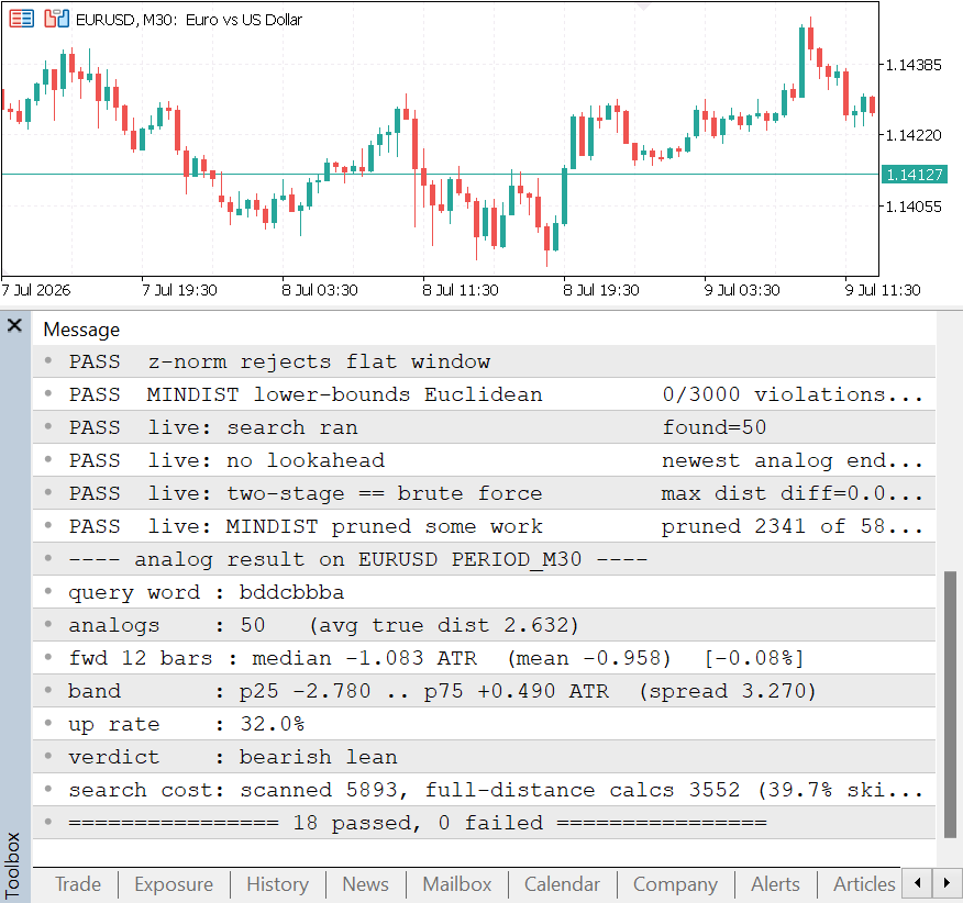
Fig. 4. The validation harness in the Experts log: the lower-bound property holds across 3000 trials, the two-stage search matches brute force exactly, and the no-lookahead guard holds on live history

The remaining checks confirm the smaller invariants: the a = 4 breakpoints land on the standard normal quartile cuts, PAA preserves the mean of the window in the non-divisible case, z-normalization produces mean zero and unit standard deviation and refuses a flat window, and the live search's newest analog ends before the query minus the horizon, the no-lookahead guard holding on real data. With every assertion passing, we could build the indicator on a foundation we had actually verified rather than merely hoped was correct.

The Indicator: Fan Cone and Verdict Panel

The indicator SAXAnalog.mq5 is where the analog search meets the trader's eye. On each new bar it encodes the current window, runs the finder over history, and renders two views: a fan cone projected into the empty space to the right of the last bar, and a verdict panel pinned to a corner. The cone is the intuition, showing where price tended to go after this shape; the panel is the honesty check, stating the sample size, the central move, the spread, and the verdict in plain numbers so a seductive-looking cone can never overstate its own support.

Drawing the cone in real price units

The forward distribution is stored in ATR multiples, which is what made precedents comparable across regimes, but a chart is drawn in price. So at draw time we convert back: each per-step median and quartile in ATR units is multiplied by the current ATR and added to the last close, which lands the cone on the real price axis at today's volatility. There is a second subtlety. The bars the cone occupies do not exist yet, so their timestamps cannot be looked up; we extrapolate them arithmetically from the last bar's time plus k times the period length in seconds. At each step we draw three segments: a solid median line and dotted 25th/75th percentile bands. Each segment starts from the previous step's endpoint to form a continuous fan.

//+------------------------------------------------------------------+
//| Draw the fan cone.                                               |
//|  The per-step distribution is in ATR units; multiply by the      |
//|  CURRENT ATR to turn it into a price offset from the last close, |
//|  so the cone sits on the real price axis. Future bar times don't |
//|  exist yet, so their timestamps are extrapolated from the last   |
//|  bar time + k * PeriodSeconds().                                 |
//+------------------------------------------------------------------+
void DrawCone(datetime lastTime,double lastClose,double curATR,color clr)
  {
   int    ps=PeriodSeconds(_Period);
   double medPrev=lastClose,p25Prev=lastClose,p75Prev=lastClose;
   datetime tPrev=lastTime;

   for(int k=1;k<=InpHorizon;k++)
     {
      SStepStat st;
      if(!g_finder.StepStats(k,st))
         break;
      datetime tk=lastTime+(datetime)(k*ps);
      double med=lastClose+st.median_atr*curATR;
      double p25=lastClose+st.p25_atr   *curATR;
      double p75=lastClose+st.p75_atr   *curATR;

      SetTrend(g_pfx+"med_"+(string)k,tPrev,medPrev,tk,med,clr,2,STYLE_SOLID);
      SetTrend(g_pfx+"p75_"+(string)k,tPrev,p75Prev,tk,p75,InpBandColor,1,STYLE_DOT);
      SetTrend(g_pfx+"p25_"+(string)k,tPrev,p25Prev,tk,p25,InpBandColor,1,STYLE_DOT);

      tPrev=tk;
      medPrev=med;
      p25Prev=p25;
      p75Prev=p75;
     }
  }

Because the cone is built from the full per-step forward paths we recorded during the search, its band genuinely widens as the horizon extends, reflecting real growth in uncertainty, rather than the straight-line triangle a naive endpoint-only projection would draw.

A panel that never clips and reads in either theme

Two small pieces of polish matter for a tool people will actually keep on their chart. First, the panel sizes itself to its own text: we measure the widest row with TextGetSize using the same font the labels use, then size the background box from that, so nothing ever spills over the edge regardless of font size or content. Second, the colors follow an InpTheme input so the panel is legible on a dark or a light chart, with the header and verdict rows carrying the verdict color and the body rows the theme's text color.

//--- theme colors
   color bgCol  =(InpTheme==THEME_LIGHT)?C'245,245,248':C'20,20,25';
   color bodyCol=(InpTheme==THEME_LIGHT)?C'40,40,45'   :clrSilver;

//--- assemble the seven rows (text + font size). Rows 0 and 6 are the
//--- accent rows; the middle five are body rows.
   string txt[7];
   int    fnt[7];
   txt[0]="SAX ANALOG FORECAST";
   fnt[0]=fHead;
   txt[1]=StringFormat("word    : %s",word);
   fnt[1]=fBody;
   txt[2]=StringFormat("analogs : %d   (avg dist %.2f)",
                       s.count,s.avg_distance);
   fnt[2]=fBody;
   txt[3]=StringFormat("fwd %2d  : median %+.2f ATR  (%+.2f%%)",
                       InpHorizon,s.median_atr,s.median_pct);
   fnt[3]=fBody;
   txt[4]=StringFormat("band    : %+.2f .. %+.2f ATR",
                       s.p25_atr,s.p75_atr);
   fnt[4]=fBody;
   txt[5]=StringFormat("up rate : %.0f%%   spread %.2f ATR",
                       100.0*s.up_rate,s.dispersion);
   fnt[5]=fBody;
   txt[6]=StringFormat("VERDICT : %s",verdict);
   fnt[6]=fHead;

//--- measure the widest row to size the box (same font as the labels)
   int maxW=0;
   for(int i=0;i<7;i++)
     {
      TextSetFont("Consolas",-fnt[i]*10);   // negative = points*10 (dpi-aware)
      uint tw=0,th=0;
      TextGetSize(txt[i],tw,th);
      if((int)tw>maxW)
         maxW=(int)tw;
     }
   int boxW=maxW+2*pad;
   int boxH=rowH*7+2*pad;

The driver, and where honesty reaches the screen

The OnCalculate handler ties it together, and it only recomputes on a new bar to keep the indicator light. It loads history, runs the finder anchored at the last closed bar, and picks a color from the verdict. Then comes the single most important line of the whole indicator: the cone is drawn only when the verdict indicates a high-conviction bullish or bearish bias. On a no-edge or too-few bar, the cone is simply not drawn, and all the trader sees is the panel stating that there is nothing here. The absence of a cone is itself the signal to stand aside.

   if(!NewBar() && prev_calculated>0)
      return(rates_total);

   double c[],atr[];
   int n=LoadHistory(c,atr);
   if(n<=0)
      return(rates_total);

//--- query ends at the newest loaded (closed) bar
   int qEnd=n-1;
   bool ok=g_finder.Find(c,atr,n,qEnd);

   SForwardStats s=g_finder.Stats();
   color clr=VerdictColor(s.verdict);

//--- last CLOSED bar anchors the cone (index 1 on the live chart)
   datetime lastTime=iTime(_Symbol,_Period,1);
   double   lastClose=iClose(_Symbol,_Period,1);
   double   curATR=(atr[n-1]>0.0)?atr[n-1]:0.0;

   ClearCone();
//--- draw the cone only when there is a high-conviction edge
   if(ok && curATR>0.0 &&
      (s.verdict==ANALOG_BULLISH || s.verdict==ANALOG_BEARISH))
      DrawCone(lastTime,lastClose,curATR,clr);

   string word=ok?g_finder.QueryWord():"-";
   DrawPanel(s,word,g_finder.VerdictText(),clr);

   ChartRedraw();
   return(rates_total);

The figure below shows the tool on EURUSD M30 at the default settings. The query window encoded to the word bddcbbba, fifty precedents were kept, and their forward distribution over the next twelve bars leaned bearish, a median of about minus one ATR with only thirty-two percent of precedents closing higher. That cleared the conviction thresholds, so the cone is drawn: a red median path sloping down, wrapped in a dotted band that widens with the horizon. The panel reports the same numbers the cone is built from, so nothing on the chart claims more than the data behind it supports.

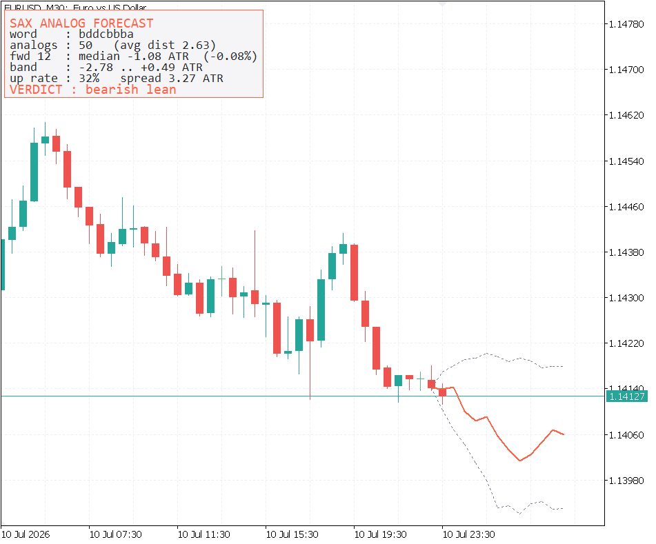
Fig. 5. The SAX analog forecaster on EURUSD M30: the fan cone projects the median path and p25-p75 band into the future, while the panel reports the statistics and the verdict behind it

Conclusion

We set out to bring Symbolic Aggregate approXimation to MQL5 honestly, and to turn it into something a discretionary trader can read at a glance. Along the way we built a genuine, reusable primitive and a tool that respects the limits of the method it is built on.

• A real SAX library. Z-normalization, PAA including the fractional non-divisible case, Gaussian breakpoints via Acklam's probit, encoding, and a MINDIST that provably lower-bounds the true distance, none of which existed on the platform before.
• A sound analog search. A two-stage prune-then-rank pipeline that uses MINDIST as a fast filter and, as we verified, returns exactly the same matches as brute force while skipping much of the work.
• Honesty by construction. A no-lookahead guard so precedents cannot see their own future, ATR-normalized outcomes so different volatility regimes are comparable, and a verdict that is allowed, and often required, to report no edge.
• A tool that reads at a glance. A fan cone for intuition and a verdict panel for the statistics behind it, with the cone suppressed whenever there is no real edge to show.

The honest conclusion is the same one we opened with. SAX is not a crystal ball for price, and this tool will tell you "no edge" more often than it tells you anything else, which is exactly as it should be on markets that are close to a random walk. Its value is in the rare, well-supported occasions when many genuine precedents lean the same way, and in the discipline of a tool that refuses to pretend otherwise. From here, the same library invites further work: SAX words as categorical features for a machine-learning model, motif and discord discovery for anomaly detection, or a Markov transition model over the word dictionary.

The programs presented in this article are intended for educational purposes only. Trading involves substantial risk, and past behavior of price shapes is not a guarantee of future results. Test any tool thoroughly on your own data and use appropriate risk management before considering it for live trading.

Getting the Source Code via MQL5 Algo Forge

All source files are attached to this article below, but the full repository is also available on MQL5 Algo Forge, the community's Git-based platform for sharing and collaborating on trading projects.

File name	Description
MQL5\Include\SAX\SAXTransform.mqh	Core SAX transform: z-normalization, PAA, Gaussian breakpoints, encoding, and the lower-bounding MINDIST
MQL5\Include\SAX\SAXAnalogs.mqh	SAX analog search: two-stage prune-then-rank matching, no-lookahead guard, ATR-normalized outcomes, and the forward-distribution verdict
MQL5\Indicators\SAX\SAXAnalog.mq5	Chart indicator drawing the forecast fan cone and the verdict panel
MQL5\Scripts\SAX\SAXValidate.mq5	Throwaway validation harness proving the transform, the lower-bound property, and the soundness of the pruning