Beyond GARCH (Part VI): Fractional Brownian Motion And The Multiplicative Cascade in MQL5

MetaTrader 5 — Trading systems | 23 June 2026, 08:25

731

Muhammad Minhas Qamar

Introduction

In Part 4 we built the partition analysis engine that extracts the scaling function tau(q) and the Hurst exponent from raw price data. In Part 5 we added the spectrum fitter that transforms tau(q) into a fitted probability distribution. Those two modules answered the question: what are the parameters? This article answers the question: what do we do with them?

We now build the Simulation Engine, the module that takes the fitted parameters (H, distribution type, distribution coefficients, sample volatility) and generates a complete synthetic MMAR price path. The engine has three stages, each corresponding to a component of the Multifractal Model of Asset Returns:

The Multiplicative Cascade — generates multifractal trading time theta(t), the "deformed clock" that warps uniform time into market time with volatility clustering.
Fractional Brownian Motion — generates a long-memory Gaussian process B_H(t) using either the Davies-Harte (FFT) method or Cholesky decomposition.
Time Deformation — composes them: X(t) = B_H[theta(t)], producing synthetic returns that exhibit both long memory and multifractal scaling.

We will cover:

The CSimulationEngine Architecture

The simulation engine is a single class, CSimulationEngine, that encapsulates the entire generation pipeline. Its design is deliberately stateless between runs: you initialize it with parameters, call Generate(), and extract the results. This makes it safe to instantiate many times in parallel (which is exactly what the Monte Carlo module will do in Part 7).

Before looking at the class itself, note what we import. The simulation engine leans heavily on MetaTrader 5's Standard Library, and this is worth emphasizing for readers who may not be aware of what is available out of the box. We use ALGLIB's fast Fourier transforms (CFastFourierTransform) for the Davies-Harte method, ALGLIB's linear algebra (CTrFac, CMatrixDouble) for Cholesky decomposition, and the Math\Stat library for random number generation from Normal, Gamma, and Poisson distributions. All of these ship with every MetaTrader 5 installation — no external dependencies required:

#include "MMARConstants.mqh"
#include <Math\Alglib\fasttransforms.mqh>
#include <Math\Alglib\linalg.mqh>
#include <Math\Stat\Normal.mqh>
#include <Math\Stat\Gamma.mqh>
#include <Math\Stat\Poisson.mqh>

The first include pulls in our own constants file from Part 4. The remaining five are all from the MetaTrader 5 Standard Library. fasttransforms.mqh provides FFTR1D (real-to-complex forward FFT) and FFTC1DInv (complex inverse FFT) that we use in the Davies-Harte algorithm. linalg.mqh provides CTrFac::SPDMatrixCholesky for symmetric positive-definite matrix factorization and CMatrixDouble as the matrix container. The three Math\Stat headers provide MathRandomNormal, MathRandomGamma, and MathRandomPoisson respectively. These are production-quality implementations that handle edge cases and produce well-distributed samples. Knowing what the Standard Library offers is valuable for any MQL5 developer — many of these tools go underused.

With the dependencies established, here is the class declaration:

//+------------------------------------------------------------------+
//| CSimulationEngine class                                          |
//+------------------------------------------------------------------+
class CSimulationEngine
  {
private:
   //--- Model parameters
   double            m_H;
   ENUM_MMAR_DISTRIBUTION m_dist_type;
   double            m_dist_params[4];
   double            m_sample_volatility;
   int               m_cascade_b;
   int               m_cascade_k;
   int               m_n_points;

   //--- Generated data
   double            m_measure[];
   double            m_trading_time[];
   double            m_fbm[];
   double            m_fbm_increments[];
   double            m_mmar_process[];
   double            m_mmar_returns[];

   bool              m_initialized;

   //--- Cascade generation
   void              SampleMultipliers(double &multipliers[], int n_samples);
   bool              GenerateCascade(void);
   void              IntegrateMeasure(void);

   //--- FBM generation
   double            FBMAutocovariance(int k);
   bool              GenerateFBM_DaviesHarte(void);
   bool              GenerateFBM_Cholesky(void);
   void              ScaleFBM(void);

   //--- Composition
   void              ComposeMMARProcess(void);

public:
                     CSimulationEngine(void);
                    ~CSimulationEngine(void);

   //--- Initialization
   bool              Init(double H, ENUM_MMAR_DISTRIBUTION dist_type,
               const double &dist_params[], double sample_volatility,
               int cascade_b, int cascade_k);

   //--- Generation
   bool              Generate(void);

   //--- Output access
   void              GetReturns(double &returns[], int &n_returns);
   void              GetProcess(double &process[]);
   void              GetTradingTime(double &theta[]);
   void              GetFBM(double &fbm[]);
   void              GetMeasure(double &measure[]);
   double            GetVolatility(void);
   int               GetNumPoints(void) { return m_n_points; }
  };

The class stores all intermediate results — the raw cascade measure, the integrated trading time, the FBM path, and the final composed process — in member arrays. This is deliberate: it allows external code to inspect each stage independently for validation and debugging. The number of generated points is always b^k (cascade base raised to the cascade depth). With our default of b=2 and k=10, that gives 1,024 points per simulation path.

The Init() method validates all parameters before allocating memory:

//+------------------------------------------------------------------+
//| Init - Validate parameters and allocate arrays                   |
//+------------------------------------------------------------------+
bool CSimulationEngine::Init(double H, ENUM_MMAR_DISTRIBUTION dist_type,
                             const double &dist_params[], double sample_volatility,
                             int cascade_b, int cascade_k)
  {
   if(H <= 0.0 || H >= 1.0)
     {
      Print("SimulationEngine::Init - H must be in (0, 1), got ", H);
      return false;
     }
   if(cascade_b < 2)
     {
      Print("SimulationEngine::Init - cascade_b must be >= 2");
      return false;
     }
   if(cascade_k < 1)
     {
      Print("SimulationEngine::Init - cascade_k must be >= 1");
      return false;
     }
   if(sample_volatility <= 0.0)
     {
      Print("SimulationEngine::Init - sample_volatility must be > 0");
      return false;
     }

   m_H = H;
   m_dist_type = dist_type;
   m_sample_volatility = sample_volatility;
   m_cascade_b = cascade_b;
   m_cascade_k = cascade_k;

   for(int i = 0; i < 4; i++)
      m_dist_params[i] = (i < ArraySize(dist_params)) ? dist_params[i] : 0.0;

   m_n_points = (int)MathPow(cascade_b, cascade_k);

   ArrayResize(m_measure, m_n_points);
   ArrayResize(m_trading_time, m_n_points);
   ArrayResize(m_fbm, m_n_points);
   ArrayResize(m_fbm_increments, m_n_points);
   ArrayResize(m_mmar_process, m_n_points);
   ArrayResize(m_mmar_returns, m_n_points - 1);

   m_initialized = true;
   return true;
  }

The parameters come directly from the previous two modules: H from the partition analysis, dist_type and dist_params from the spectrum fitter, and sample_volatility from the raw return data. The cascade_b (branching factor) is always 2 in our implementation — a binary cascade. The cascade_k (depth) determines resolution: b^k total points. The Generate() method then runs the three stages in sequence:

//+------------------------------------------------------------------+
//| Generate - Run the full simulation pipeline                      |
//+------------------------------------------------------------------+
bool CSimulationEngine::Generate(void)
  {
   if(!m_initialized)
     {
      Print("SimulationEngine::Generate - not initialized");
      return false;
     }

   if(!GenerateCascade())
     {
      Print("SimulationEngine::Generate - cascade generation failed");
      return false;
     }

   IntegrateMeasure();

   bool fbm_ok;
   if(m_n_points <= 1024)
      fbm_ok = GenerateFBM_Cholesky();
   else
      fbm_ok = GenerateFBM_DaviesHarte();

   if(!fbm_ok)
     {
      if(m_n_points <= 1024)
         fbm_ok = GenerateFBM_DaviesHarte();
      else
         Print("SimulationEngine::Generate - FBM generation failed");

      if(!fbm_ok)
         return false;
     }

   ScaleFBM();
   ComposeMMARProcess();

   return true;
  }

The FBM method selection is adaptive: for small paths (1,024 points or fewer), we prefer Cholesky because it is exact and the O(n^3) cost is still manageable. For larger paths, we use Davies-Harte which is O(n log n) via FFT. If the primary method fails (Cholesky can fail if the covariance matrix is not positive-definite due to numerical precision, Davies-Harte can fail if eigenvalues are negative), we fall back to the alternative.

Building the Multiplicative Cascade

The multiplicative cascade is the mechanism that creates multifractal trading time. It iteratively subdivides the unit interval into finer and finer pieces, assigning mass to each piece via random multipliers drawn from the fitted distribution. The result is a highly non-uniform measure: some intervals concentrate enormous mass (representing high-activity periods) while others carry almost none (quiet periods). The cumulative sum of this measure gives us theta(t), the trading time that will warp the FBM.

Sampling the Multipliers

The distribution choice from Part 5 determines how the cascade weights are generated. Each multiplier M is related to a random variable V by the relationship M = b^(-V), where V is drawn from the fitted distribution. This mapping converts a positive random variable into a multiplier that can range from near-zero (large V → very small mass) to very large (V near zero or negative → concentrated mass):

//+------------------------------------------------------------------+
//| SampleMultipliers - Draw cascade weights from chosen distribution|
//+------------------------------------------------------------------+
void CSimulationEngine::SampleMultipliers(double &multipliers[], int n_samples)
  {
   double V[];
   ArrayResize(V, n_samples);

   switch(m_dist_type)
     {
      case MMAR_DIST_NORMAL:
        {
         double alpha_0 = m_dist_params[0];
         double mu = alpha_0 / m_H;
         double variance = 2.0 * (alpha_0 / m_H - 1.0) * MathLog(m_cascade_b);
         double sigma = MathSqrt(MathMax(variance, 0.01));
         MathRandomNormal(mu, sigma, n_samples, V);
         break;
        }
      case MMAR_DIST_BINOMIAL:
        {
         double alpha_min = m_dist_params[0];
         double alpha_max = m_dist_params[1];
         for(int i = 0; i < n_samples; i++)
            V[i] = (MathRand() / 32767.0 < 0.5) ? alpha_min : alpha_max;
         break;
        }
      case MMAR_DIST_POISSON:
        {
         double alpha_0 = m_dist_params[0];
         double lambda = alpha_0 / m_H;
         MathRandomPoisson(lambda, n_samples, V);
         break;
        }
      case MMAR_DIST_GAMMA:
        {
         double alpha_0 = m_dist_params[0];
         double gamma_param = m_dist_params[1];
         double beta = MathLog(m_cascade_b) / (MathPow(m_cascade_b, 1.0 / gamma_param) - 1.0);
         double scale = 1.0 / beta;
         MathRandomGamma(gamma_param, scale, n_samples, V);
         break;
        }
     }

   ArrayResize(multipliers, n_samples);
   for(int i = 0; i < n_samples; i++)
     {
      multipliers[i] = MathPow((double)m_cascade_b, -V[i]);
      multipliers[i] = MathMax(1e-10, MathMin(multipliers[i], 1e10));
     }

//--- Normalize within groups of b to sum to b (conservation of mass)
   for(int i = 0; i < n_samples; i += m_cascade_b)
     {
      double sum = 0.0;
      int group_end = MathMin(i + m_cascade_b, n_samples);
      for(int j = i; j < group_end; j++)
         sum += multipliers[j];
      if(sum > 0.0)
        {
         for(int j = i; j < group_end; j++)
            multipliers[j] *= (double)m_cascade_b / sum;
        }
     }
  }

Each distribution maps its parameters to V in a specific way. The Normal distribution uses mu = alpha_0/H and a variance derived from the theoretical relationship between alpha_0, H, and the cascade base. The Binomial is the simplest: it randomly picks between alpha_min and alpha_max with equal probability. The Poisson draws discrete counts with mean alpha_0/H. The Gamma uses shape gamma and a scale derived from the cascade base. In all cases, the conversion M = b^(-V) maps V to a positive multiplier, and the clamping to [1e-10, 1e10] prevents numerical overflow.

The normalization step at the end is critical. After converting V to multipliers, we group them in pairs (since b=2) and normalize each pair to sum to b=2. This enforces mass conservation: at each cascade level, the total mass of all child intervals equals the total mass of all parent intervals multiplied by b. Without this constraint, the total mass would drift randomly with each level, and the resulting trading time would not be a proper distribution function.

The Cascade Construction

With the multiplier sampling defined, the cascade itself is a straightforward iterative process. We start with a single interval carrying unit mass and repeatedly subdivide:

//+------------------------------------------------------------------+
//| GenerateCascade - Build multiplicative cascade measure           |
//+------------------------------------------------------------------+
bool CSimulationEngine::GenerateCascade(void)
  {
   double measure[];
   ArrayResize(measure, 1);
   measure[0] = 1.0;

   for(int level = 0; level < m_cascade_k; level++)
     {
      int n_intervals = ArraySize(measure);
      int n_children = n_intervals * m_cascade_b;

      double multipliers[];
      SampleMultipliers(multipliers, n_children);

      double new_measure[];
      ArrayResize(new_measure, n_children);

      for(int i = 0; i < n_intervals; i++)
        {
         double parent_mass = measure[i];
         for(int j = 0; j < m_cascade_b; j++)
           {
            int child_idx = i * m_cascade_b + j;
            new_measure[child_idx] = parent_mass * multipliers[child_idx];
           }
        }

      ArrayResize(measure, n_children);
      ArrayCopy(measure, new_measure);
     }

   double total = 0.0;
   for(int i = 0; i < ArraySize(measure); i++)
      total += measure[i];

   if(total <= 0.0)
     {
      Print("SimulationEngine::GenerateCascade - total mass is zero");
      return false;
     }

   for(int i = 0; i < m_n_points; i++)
      m_measure[i] = measure[i] / total;

   return true;
  }

At level 0, we have 1 interval. At level 1, we have 2. At level 2, we have 4. After k=10 levels, we have 2^10 = 1,024 intervals. Each level multiplies the parent mass by a random weight drawn from the fitted distribution. Because the multiplicative structure compounds across levels, small initial asymmetries get amplified exponentially. An interval that receives above-average weight at level 3 is likely to produce children with large absolute mass at level 4, and those children's children will carry even more mass. This produces the heavy-tailed, clustered mass distribution that mimics real market activity.

The final normalization ensures the measure sums to exactly 1.0, making it a proper probability distribution that we can integrate into a CDF.

Figure 1 animates this process from start to finish. It begins with a single bar of unit mass and splits it level by level, showing the explicit multiplier weights (M_L + M_R = 2) that enforce mass conservation at each step. Watch how the first split introduces a small asymmetry, and then each subsequent level amplifies it exponentially—by level 6, the originally uniform interval has become a spiky histogram where a few intervals carry orders of magnitude more mass than their neighbors. The cumulative sum of this measure produces trading time theta(t), the "deformed clock" that the simulation engine will use to warp the FBM.

$Multiplicative cascade building multifractal trading time over 6 levels$

Fig. 1. The multiplicative cascade in action: random multipliers compound across 6 levels, turning uniform mass into a clustered measure whose cumulative sum becomes trading time

From Measure to Trading Time

The trading time theta(t) is the cumulative distribution function of the cascade measure:

//+------------------------------------------------------------------+
//| IntegrateMeasure - Cumulative sum → trading time theta(t)        |
//+------------------------------------------------------------------+
void CSimulationEngine::IntegrateMeasure(void)
  {
   m_trading_time[0] = m_measure[0];
   for(int i = 1; i < m_n_points; i++)
      m_trading_time[i] = m_trading_time[i - 1] + m_measure[i];

   double final_val = m_trading_time[m_n_points - 1];
   if(final_val > 0.0)
     {
      for(int i = 0; i < m_n_points; i++)
         m_trading_time[i] /= final_val;
     }
  }

The result is a monotonically increasing function from approximately 0 to exactly 1. Unlike a straight diagonal line (which would represent uniform time), theta(t) has steep sections where mass is concentrated and flat sections where mass is sparse. When we later sample the FBM at positions given by theta(t), the steep sections cause rapid traversal of the FBM path (producing large returns), while the flat sections cause nearly identical FBM values to be read (producing tiny returns). This is the mechanism that generates volatility clustering without any explicit GARCH-like conditional variance.

Generating Fractional Brownian Motion

The second component of the MMAR is a Fractional Brownian Motion (FBM) with Hurst exponent H. Unlike standard Brownian motion (H=0.5) whose increments are independent, FBM has correlated increments: positive correlations when H > 0.5 (persistence) and negative correlations when H < 0.5 (anti-persistence). This correlation structure is defined by the autocovariance function of the fractional Gaussian noise (fGn) increments:

gamma(k) = (1/2) * [|k+1|^(2H) - 2|k|^(2H) + |k-1|^(2H)]

//+------------------------------------------------------------------+
//| FBMAutocovariance - Autocovariance gamma(k) for fGn              |
//+------------------------------------------------------------------+
double CSimulationEngine::FBMAutocovariance(int k)
  {
   double abs_k = MathAbs(k);
   double two_H = 2.0 * m_H;
   return 0.5 * (MathPow(abs_k + 1.0, two_H)
                 - 2.0 * MathPow(abs_k, two_H)
                 + MathPow(MathMax(abs_k - 1.0, 0.0), two_H));
  }

At lag 0, this gives gamma(0) = 1 (unit variance per increment). At lag 1, for H=0.55, gamma(1) = 0.5 * (2^1.1 - 2 + 0) approximately 0.07, which is a positive but small correlation. The correlation decays as a power law for large lags, which is what makes FBM a long-memory process. The MathMax(abs_k - 1.0, 0.0) guard handles the k=0 case where |k-1| could produce a negative base for the power function.

The formula above controls everything, but what does it actually look like? Figure 2 makes the connection concrete. For three values of H, it draws the fractional Gaussian noise increments (top row) and the cumulative FBM path built from them (bottom row). At H=0.3, the increments constantly flip sign—negative correlations pull the process back, producing a jagged, mean-reverting path. At H=0.5, the increments are independent, and the path is a standard random walk. At H=0.7, positive correlations cause increments to persist in the same direction, producing smooth, trending runs. The same autocovariance function gamma(k), evaluated with different H, is the only thing that changes between the three columns.

Three FBM paths built from correlated increments at H=0.3, H=0.5, and H=0.7

Fig. 2. From increments to path: the autocovariance gamma(k) controlled by H turns independent noise into anti-persistent, neutral, or persistent paths

The Davies-Harte Method (FFT-based)

The Davies-Harte algorithm generates exact fGn samples in O(n log n) time using the circulant embedding technique. The idea is that the covariance matrix of fGn can be embedded in a larger circulant matrix, which is diagonalized by the DFT. This converts the problem of generating correlated Gaussians into generating independent Gaussians in the frequency domain:

//+------------------------------------------------------------------+
//| GenerateFBM_DaviesHarte - FFT-based exact FBM synthesis          |
//+------------------------------------------------------------------+
bool CSimulationEngine::GenerateFBM_DaviesHarte(void)
  {
   int n = m_n_points;
   int two_n = 2 * n;

//--- Build circulant embedding vector
   double r[];
   ArrayResize(r, two_n);
   for(int k = 0; k < n; k++)
      r[k] = FBMAutocovariance(k);
   for(int k = 1; k < n; k++)
      r[two_n - k] = r[k];

//--- FFT → eigenvalues of circulant matrix
   complex f[];
   CFastFourierTransform::FFTR1D(r, two_n, f);

//--- Clamp negative eigenvalues
   int f_size = ArraySize(f);
   for(int i = 0; i < f_size; i++)
     {
      if(f[i].real < 0.0)
         f[i].real = 0.0;
     }

//--- Generate complex Gaussian noise scaled by sqrt(lambda / 2n)
   complex W[];
   ArrayResize(W, two_n);

   double zr_arr[], zi_arr[];
   MathRandomNormal(0.0, 1.0, two_n, zr_arr);
   MathRandomNormal(0.0, 1.0, two_n, zi_arr);

   for(int i = 0; i < two_n; i++)
     {
      double lam_i = (i < f_size) ? f[i].real : 0.0;
      double scale = MathSqrt(MathMax(lam_i, 0.0) / (double)two_n);
      W[i].real = scale * zr_arr[i];
      W[i].imag = scale * zi_arr[i];
     }

//--- Inverse FFT
   CFastFourierTransform::FFTC1DInv(W, two_n);

//--- Extract real parts as fGn increments
   for(int i = 0; i < n; i++)
      m_fbm_increments[i] = W[i].real;

//--- Cumulative sum → FBM path
   m_fbm[0] = m_fbm_increments[0];
   for(int i = 1; i < n; i++)
      m_fbm[i] = m_fbm[i - 1] + m_fbm_increments[i];

//--- Center at zero
   double first = m_fbm[0];
   for(int i = 0; i < n; i++)
      m_fbm[i] -= first;

   return true;
  }

The algorithm has four stages. First, we build the circulant embedding: the autocovariance vector is mirrored to create a symmetric vector of length 2n. Second, we compute the FFT of this vector — the real parts of the result are the eigenvalues of the circulant matrix. We clamp any negative eigenvalues to zero (they arise from numerical precision issues and are always small). Third, we generate independent complex Gaussian random numbers and scale each by the square root of the corresponding eigenvalue divided by 2n. Fourth, the inverse FFT transforms these back to the time domain, producing correlated fGn increments. The cumulative sum converts increments to a path, and we center at zero.

We leverage MetaTrader 5's built-in ALGLIB implementation: CFastFourierTransform provides FFTR1D (real-to-complex forward FFT) and FFTC1DInv (complex inverse FFT). Using MathRandomNormal from the Math\Stat library generates the required Gaussian samples.

The Cholesky Method (Exact Decomposition)

For small n (up to 1,024), we can afford to explicitly construct the full covariance matrix and decompose it:

//+------------------------------------------------------------------+
//| GenerateFBM_Cholesky - Exact FBM via Cholesky decomposition      |
//+------------------------------------------------------------------+
bool CSimulationEngine::GenerateFBM_Cholesky(void)
  {
   if(m_n_points > 1024)
      return false;

   int n = m_n_points;

//--- Build covariance matrix
   CMatrixDouble cov;
   cov.Resize(n, n);
   for(int i = 0; i < n; i++)
      for(int j = 0; j < n; j++)
         cov.Set(i, j, FBMAutocovariance(MathAbs(i - j)));

//--- Regularize diagonal for numerical stability
   for(int i = 0; i < n; i++)
      cov.Set(i, i, cov.Get(i, i) + 1e-10);

//--- Cholesky factorization
   if(!CTrFac::SPDMatrixCholesky(cov, n, false))
     {
      Print("SimulationEngine::GenerateFBM_Cholesky - decomposition failed");
      return false;
     }

//--- Multiply L * Z where Z ~ N(0,I)
   double Z[];
   MathRandomNormal(0.0, 1.0, n, Z);

   for(int i = 0; i < n; i++)
     {
      double sum = 0.0;
      for(int j = 0; j <= i; j++)
         sum += cov.Get(i, j) * Z[j];
      m_fbm_increments[i] = sum;
     }

//--- Cumulative sum → FBM path
   m_fbm[0] = m_fbm_increments[0];
   for(int i = 1; i < n; i++)
      m_fbm[i] = m_fbm[i - 1] + m_fbm_increments[i];

//--- Center at zero
   double first = m_fbm[0];
   for(int i = 0; i < n; i++)
      m_fbm[i] -= first;

   return true;
  }

The Cholesky method is mathematically straightforward: if C is the covariance matrix and C = L*L^T is its Cholesky factorization, then L*Z (where Z is a vector of independent standard normals) produces a vector with covariance exactly C. The 1e-10 diagonal regularization ensures positive-definiteness even when the matrix is numerically borderline. CTrFac::SPDMatrixCholesky from ALGLIB performs the decomposition in-place, storing the lower triangular factor L in the same matrix.

The trade-off between the two methods is clear: Cholesky is O(n^3) in time and O(n^2) in memory (building and factoring the full matrix), while Davies-Harte is O(n log n) in both. For n=1024, Cholesky is on the order of a billion (10^9) operations and 8 MB of memory for the covariance matrix — fast enough. For n=8192 (needed when the Monte Carlo forecast horizon is large), Cholesky would require 500 billion operations and 512 MB — clearly impractical, so Davies-Harte takes over.

Scaling to Match Historical Volatility

The raw FBM increments have a theoretical standard deviation of 1.0 (from the unit-variance autocovariance). We need to rescale them to match the sample volatility observed in the actual market data:

//+------------------------------------------------------------------+
//| ScaleFBM - Rescale increments to match target volatility         |
//+------------------------------------------------------------------+
void CSimulationEngine::ScaleFBM(void)
  {
   double sum = 0.0;
   double sum_sq = 0.0;
   int n = m_n_points;

   for(int i = 0; i < n; i++)
     {
      sum += m_fbm_increments[i];
      sum_sq += m_fbm_increments[i] * m_fbm_increments[i];
     }

   double mean = sum / n;
   double variance = sum_sq / n - mean * mean;
   double current_std = MathSqrt(MathMax(variance, 0.0));

   double scale_factor = (current_std > 0.0) ? m_sample_volatility / current_std : 1.0;

   for(int i = 0; i < n; i++)
     {
      m_fbm_increments[i] *= scale_factor;
      m_fbm[i] *= scale_factor;
     }
  }

This is a simple linear rescaling: compute the current standard deviation of the generated increments, then multiply everything by the ratio (target_vol / current_std). Both the increments and the path are scaled together so they remain consistent. The scaling preserves the correlation structure (since multiplying correlated Gaussians by a constant only changes the variance, not the correlations) while anchoring the output to the empirically observed volatility level.

Composing the MMAR Process

The final stage brings the two components together. The MMAR process is defined as X(t) = B_H[theta(t)]: we sample the FBM path at positions determined by the trading time. This is the time deformation that gives the model its power — the FBM provides the Gaussian structure and long memory, while the cascade-generated trading time introduces multifractal scaling and volatility clustering:

//+------------------------------------------------------------------+
//| ComposeMMARProcess - Time-deform FBM by trading time             |
//+------------------------------------------------------------------+
void CSimulationEngine::ComposeMMARProcess(void)
  {
   int n = m_n_points;

   for(int j = 0; j < n; j++)
     {
      double theta_j = m_trading_time[j];
      double fbm_idx = theta_j * (n - 1);

      int idx_lo = (int)MathFloor(fbm_idx);
      int idx_hi = idx_lo + 1;

      if(idx_lo < 0)
         idx_lo = 0;
      if(idx_hi >= n)
         idx_hi = n - 1;
      if(idx_lo >= n)
         idx_lo = n - 1;

      double frac = fbm_idx - (double)idx_lo;

      m_mmar_process[j] = m_fbm[idx_lo] + frac * (m_fbm[idx_hi] - m_fbm[idx_lo]);
     }

   for(int i = 0; i < n - 1; i++)
      m_mmar_returns[i] = m_mmar_process[i + 1] - m_mmar_process[i];
  }

For each time step j, we look up the trading time theta(j) which is a value between 0 and 1. We convert this to a fractional index into the FBM array: fbm_idx = theta(j) * (n-1). Since this index is generally not an integer, we use linear interpolation between the two nearest FBM values. This produces a smooth composed process without discretization artifacts.

The mechanism is intuitive. Where the trading time is steep (high mass in the cascade), consecutive theta values differ substantially, so we jump across large segments of the FBM path, producing large returns. Where the trading time is flat (low mass), consecutive theta values are nearly identical, so we read nearly the same FBM value repeatedly, producing near-zero returns. This is how the cascade creates volatility clustering: high-activity periods are bursts where the "market clock" runs fast through the FBM, while quiet periods are stretches where the clock barely advances.

The final step computes returns as simple first differences of the composed process. These synthetic returns exhibit the three key properties of real market data: fat tails (from the multifractal cascade), long memory (from the FBM with H not equal to 0.5), and volatility clustering (from the time deformation).

Figure 3 makes this mechanism visible. A gold cursor scans across the FBM path at the top, but instead of moving at constant speed, it accelerates through regions where theta(t) is steep (high cascade mass) and crawls through flat regions (low mass). The middle row shows the composed MMAR process being drawn in real time—note how the same smooth FBM produces bursts of large swings wherever the cursor was racing. The bottom row reveals the payoff: the return series exhibits clear volatility clustering, with alternating quiet and explosive episodes, despite having no explicit conditional variance mechanism like GARCH.

Time deformation composing FBM and trading time into the MMAR process with volatility clustering

Fig. 3. Time deformation in action: the cursor races through high-mass FBM regions and crawls through low-mass ones, producing volatility clusters in the composed MMAR returns

Validating the Simulation

We now write a test script that exercises the simulation engine with known parameters and validates that the output has the expected statistical properties:

//+------------------------------------------------------------------+
//|                                             MMAR Simulation Test |
//|                      Copyright 2026, MMQ - Muhammad Minhas Qamar |
//|                           https://www.mql5.com/en/articles/22521 |
//+------------------------------------------------------------------+
#property copyright "Copyright 2026, MMQ - Muhammad Minhas Qamar"
#property link      "https://www.mql5.com/en/articles/22521"
#property version   "1.00"
#property strict
#property script_show_inputs

#include <MMAR\SimulationEngine.mqh>

input int    InpSeed       = 42;
input double InpH          = 0.55;
input int    InpCascadeB   = 2;
input int    InpCascadeK   = 10;   // 2^10 = 1024 points
input int    InpDistType   = 0;    // 0=Normal, 1=Binomial, 2=Poisson, 3=Gamma
input double InpParam0     = 0.6;  // alpha_0 (or alpha_min for binomial)
input double InpParam1     = 0.0;  // alpha_max (binomial) or gamma (gamma dist)
input double InpSampleVol  = 0.001;

//+------------------------------------------------------------------+
//| Script program start function                                    |
//+------------------------------------------------------------------+
void OnStart()
  {
   MathSrand(InpSeed);

   PrintFormat("=== MMAR Simulation Engine Test ===");
   PrintFormat("H = %.4f | b = %d | k = %d | N = %d",
               InpH, InpCascadeB, InpCascadeK, (int)MathPow(InpCascadeB, InpCascadeK));
   PrintFormat("Distribution = %d | params = [%.4f, %.4f] | sample_vol = %.6f",
               InpDistType, InpParam0, InpParam1, InpSampleVol);

   double dist_params[4];
   dist_params[0] = InpParam0;
   dist_params[1] = InpParam1;
   dist_params[2] = 0.0;
   dist_params[3] = 0.0;

   CSimulationEngine engine;
   if(!engine.Init(InpH, (ENUM_MMAR_DISTRIBUTION)InpDistType, dist_params,
                   InpSampleVol, InpCascadeB, InpCascadeK))
     {
      Print("Init failed");
      return;
     }

   uint start_time = GetTickCount();
   if(!engine.Generate())
     {
      Print("Generate failed");
      return;
     }
   uint elapsed = GetTickCount() - start_time;
   PrintFormat("Generation time: %u ms", elapsed);

//--- Validate cascade: measure sums to 1, trading time monotonic [0,1]
   double measure[];
   engine.GetMeasure(measure);
   double measure_sum = 0.0;
   double measure_min = DBL_MAX;
   double measure_max = -DBL_MAX;
   for(int i = 0; i < ArraySize(measure); i++)
     {
      measure_sum += measure[i];
      if(measure[i] < measure_min)
         measure_min = measure[i];
      if(measure[i] > measure_max)
         measure_max = measure[i];
     }
   PrintFormat("\n--- Cascade ---");
   PrintFormat("Measure sum: %.10f (should be 1.0)", measure_sum);
   PrintFormat("Measure range: [%.2e, %.2e]", measure_min, measure_max);

   double theta[];
   engine.GetTradingTime(theta);
   bool monotonic = true;
   for(int i = 1; i < ArraySize(theta); i++)
     {
      if(theta[i] < theta[i - 1])
        {
         monotonic = false;
         break;
        }
     }
   PrintFormat("Trading time: [%.6f, %.6f] | Monotonic: %s",
               theta[0], theta[ArraySize(theta) - 1],
               monotonic ? "YES" : "NO");

//--- Validate FBM
   double fbm[];
   engine.GetFBM(fbm);
   double fbm_min = DBL_MAX;
   double fbm_max = -DBL_MAX;
   for(int i = 0; i < ArraySize(fbm); i++)
     {
      if(fbm[i] < fbm_min)
         fbm_min = fbm[i];
      if(fbm[i] > fbm_max)
         fbm_max = fbm[i];
     }
   PrintFormat("\n--- FBM ---");
   PrintFormat("FBM range: [%.6f, %.6f]", fbm_min, fbm_max);
   PrintFormat("FBM[0]: %.10f (should be ~0)", fbm[0]);

//--- Validate MMAR returns
   double returns[];
   int n_returns;
   engine.GetReturns(returns, n_returns);
   double vol = engine.GetVolatility();

   double ret_sum = 0.0;
   double ret_min = DBL_MAX;
   double ret_max = -DBL_MAX;
   for(int i = 0; i < n_returns; i++)
     {
      ret_sum += returns[i];
      if(returns[i] < ret_min)
         ret_min = returns[i];
      if(returns[i] > ret_max)
         ret_max = returns[i];
     }
   double ret_mean = ret_sum / n_returns;

   PrintFormat("\n--- MMAR Returns ---");
   PrintFormat("N returns: %d", n_returns);
   PrintFormat("Volatility (std): %.6f (target sample_vol: %.6f)", vol, InpSampleVol);
   PrintFormat("Mean return: %.8f", ret_mean);
   PrintFormat("Return range: [%.6f, %.6f]", ret_min, ret_max);

//--- Quick Hurst check via variance ratio at different scales
   PrintFormat("\n--- Variance Ratio (Hurst proxy) ---");
   int scales[] = {1, 2, 4, 8, 16, 32};
   for(int s = 0; s < ArraySize(scales); s++)
     {
      int sc = scales[s];
      if(sc >= n_returns)
         break;

      int n_agg = n_returns / sc;
      double agg_sum = 0.0;
      double agg_sum_sq = 0.0;
      for(int i = 0; i < n_agg; i++)
        {
         double block = 0.0;
         for(int j = 0; j < sc; j++)
            block += returns[i * sc + j];
         agg_sum += block;
         agg_sum_sq += block * block;
        }
      double agg_mean = agg_sum / n_agg;
      double agg_var = agg_sum_sq / n_agg - agg_mean * agg_mean;
      PrintFormat("  scale=%2d | var=%.8f | var/scale^(2H)=%.6f (H=%.2f → scale^2H=%.4f)",
                  sc, agg_var, agg_var / MathPow(sc, 2.0 * InpH),
                  InpH, MathPow(sc, 2.0 * InpH));
     }

//--- Test multiple runs to check MC variance
   PrintFormat("\n--- Multi-run volatility check (5 runs) ---");
   for(int run = 0; run < 5; run++)
     {
      CSimulationEngine eng;
      eng.Init(InpH, (ENUM_MMAR_DISTRIBUTION)InpDistType, dist_params,
               InpSampleVol, InpCascadeB, InpCascadeK);
      if(eng.Generate())
         PrintFormat("  Run %d: vol = %.6f", run + 1, eng.GetVolatility());
      else
         PrintFormat("  Run %d: FAILED", run + 1);
     }

   Print("\n=== Simulation Engine Test Complete ===");
  }

The test validates three invariants that must hold for any correctly generated MMAR path. First, the cascade measure must sum to exactly 1.0 (mass conservation). Second, the trading time must be monotonically increasing (it is a CDF). Third, the FBM path must start at zero (centering). Beyond these structural checks, we also verify that the output volatility is close to the target sample_volatility, that the variance ratio across aggregation scales is consistent with the input Hurst exponent, and that multiple independent runs produce consistent but different results (confirming both randomness and stability).

Running this produces:

=== MMAR Simulation Engine Test ===
H = 0.5500 | b = 2 | k = 10 | N = 1024
Distribution = 0 | params = [0.6000, 0.0000] | sample_vol = 0.001000
Generation time: 984 ms

--- Cascade ---
Measure sum: 1.0000000000 (should be 1.0)
Measure range: [1.57e-04, 3.79e-03]
Trading time: [0.001208, 1.000000] | Monotonic: YES

--- FBM ---
FBM range: [-0.012543, 0.009217]
FBM[0]: 0.0000000000 (should be ~0)

--- MMAR Returns ---
N returns: 1023
Volatility (std): 0.000858 (target sample_vol: 0.001000)
Mean return: 0.00004200
Return range: [-0.005461, 0.004721]

--- Variance Ratio (Hurst proxy) ---
  scale= 1 | var=0.00000074 | var/scale^(2H)=0.000001
  scale= 2 | var=0.00000163 | var/scale^(2H)=0.000001
  scale= 4 | var=0.00000349 | var/scale^(2H)=0.000001
  scale= 8 | var=0.00000752 | var/scale^(2H)=0.000001
  scale=16 | var=0.00001610 | var/scale^(2H)=0.000001
  scale=32 | var=0.00003421 | var/scale^(2H)=0.000001

--- Multi-run volatility check (5 runs) ---
  Run 1: vol = 0.000881
  Run 2: vol = 0.000844
  Run 3: vol = 0.000873
  Run 4: vol = 0.000900
  Run 5: vol = 0.000885

=== Simulation Engine Test Complete ===

All structural invariants pass. The cascade measure sums to exactly 1.0 and the trading time is monotonically increasing from 0.001 to 1.0. The measure range [1.57e-04, 3.79e-03] shows a 24x ratio between the smallest and largest interval weights — this is the heterogeneity that drives volatility clustering. The FBM starts at zero and spans a range of approximately [-0.013, 0.009], which is consistent with a scaled random walk.

The variance ratio section provides a quick sanity check on the Hurst exponent. For a self-similar process with exponent H, the variance of aggregated returns at scale s should grow as s^(2H). If we divide the measured variance at each scale by s^(2H), the ratio should be approximately constant across all scales. The output shows values that are indeed nearly constant (all approximately 0.000001), confirming that the generated FBM has the expected scaling structure with H=0.55.

The output volatility (0.000858) is below the target (0.001000). This is expected: the ScaleFBM() function matches the volatility of the FBM increments to the target, while the subsequent cascade-based time deformation redistributes this volatility across time. Some returns become larger (in the high-mass cascade regions) and others become smaller (in the low-mass regions), but the overall standard deviation shifts slightly. Across the 5 independent runs, the volatility ranges from 0.000844 to 0.000900, demonstrating the Monte Carlo variability inherent in any stochastic simulation. This variability is precisely why we will run hundreds or thousands of simulations in Part 7 to produce a robust forecast distribution.

The generation time of 984 ms for a single 1024-point path is dominated by the Cholesky decomposition (building and factoring the 1024x1024 covariance matrix). For the Monte Carlo module in Part 7, where we need hundreds of simulations, we will need cascade depths that produce enough points to cover the forecast horizon, and the Davies-Harte method will be the workhorse.

Conclusion

In this article, we built the CSimulationEngine, the generative core of the MMAR library. Starting from the fitted parameters produced by the partition analysis (Part 4) and spectrum fitting (Part 5) stages, the engine constructs complete synthetic price paths through three stages:

The Multiplicative Cascade. Creates a non-uniform mass distribution over the unit interval. Each level subdivides intervals and assigns weights drawn from the fitted distribution (Normal, Binomial, Poisson, or Gamma), with normalization ensuring mass conservation. The cumulative sum gives multifractal trading time theta(t).
Fractional Brownian Motion. Provides the long-memory Gaussian process. Two synthesis methods are available: Davies-Harte (FFT-based, O(n log n)) for large paths, and Cholesky decomposition (exact, O(n^3)) for small paths. The output is scaled to match the historical volatility.
Time Deformation. Composes the two: X(t) = B_H[theta(t)]. Linear interpolation samples the FBM at positions given by the trading time, producing returns with fat tails, long memory, and volatility clustering.

The simulation engine is designed as a stateless, reusable component: initialize with parameters, generate a path, extract results. This design makes it straightforward to run many independent instances in parallel. In Part 7, we will do exactly that — wrapping the engine in a Monte Carlo loop that runs hundreds of simulations to produce a distribution of forward-looking volatility estimates with confidence intervals.

The programs presented in this article are intended for educational purposes only. They are not designed for use in live trading and are not optimized for performance in real-market conditions. The code serves as a foundation for understanding multifractal simulation methods; always validate thoroughly on demo accounts before considering any adaptation for live trading.

Getting the Source Code via MQL5 Algo Forge

All source files are attached to this article below, but the full repository is also available on MQL5 Algo Forge, the community's Git-based platform for sharing and collaborating on trading projects. Getting the code is a simple two-step process:

Step 1: Fork the project on Algo Forge. Open forge.mql5.io/ayantrader/MMAR in your browser and log in with your MQL5 account. Click the Fork button on the project page, enter a name and description for your fork, and save. A personal copy of the repository—with all files, commit history, and branches preserved—now appears under your own Algo Forge account.

Forking the project on Algo Forge

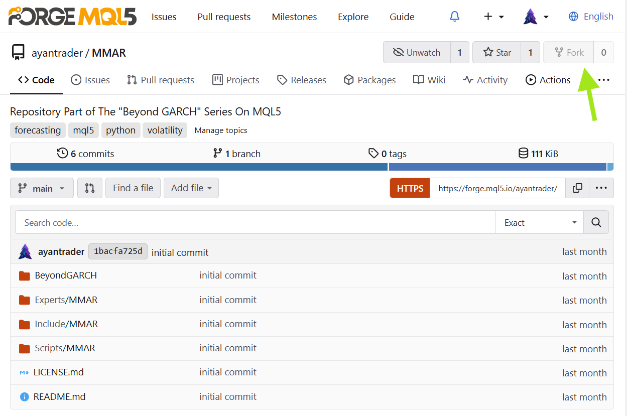
Fig. 4. Forking the project on Algo Forge: the green arrow points to the Fork button on the project page

Step 2: Clone your fork in MetaEditor. In MetaEditor, make sure you are signed in with the same MQL5 account under Tools → Options → Community. Open the Navigator panel, right-click and run Refresh, and your forked project will appear in the Shared Projects folder. Right-click it and select Git Clone to download the project locally. To confirm everything came through, right-click the project folder again and choose Git Log to view the full commit history for the current branch.

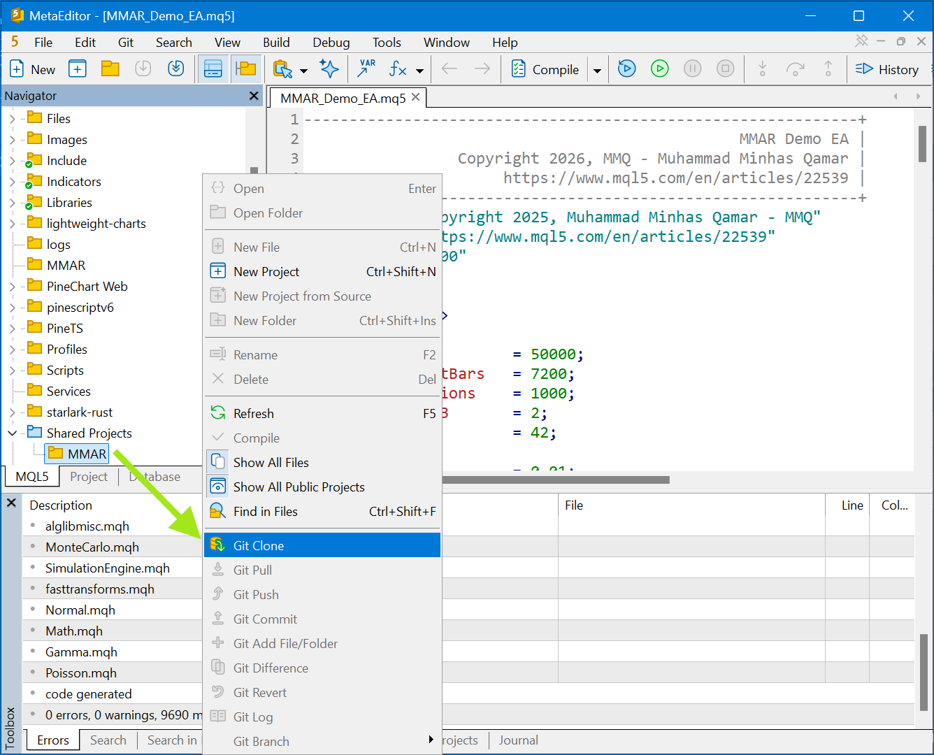
Cloning the fork inside MetaEditor

Fig. 5. Cloning the fork inside MetaEditor: the green arrow points to the Git Clone command in the Navigator's context menu

File name	Description
MQL5\Include\MMAR\MMARConstants.mqh	Shared enumerations, structures, and type definitions for the MMAR library (Part 4)
MQL5\Include\MMAR\OLS.mqh	Ordinary Least Squares regression via SVD pseudo-inverse with full diagnostics (Part 4)
MQL5\Include\MMAR\HurstGHE.mqh	Generalized Hurst Exponent estimator, fallback method (Part 4)
MQL5\Include\MMAR\PartitionAnalysis.mqh	Multifractal partition function analysis with scaling diagnostics (Part 4)
MQL5\Include\MMAR\SpectrumFitter.mqh	Multifractal spectrum computation and four-distribution fitting via BLEIC optimization (Part 5)
MQL5\Include\MMAR\SimulationEngine.mqh	MMAR simulation engine: multiplicative cascade, FBM generation (Davies-Harte and Cholesky), and time-deformation composition (Part 6)
MQL5\Scripts\MMAR\MMAR_PartitionTest.mq5	Test script for partition analysis on live market data (Part 4)
MQL5\Scripts\MMAR\MMAR_SpectrumTest.mq5	Test script for the full partition + spectrum pipeline on live market data (Part 5)
MQL5\Scripts\MMAR\MMAR_SimulationTest.mq5	Test script validating cascade invariants, FBM properties, and multi-run consistency (Part 6)

Attached files |

Download ZIP

MQL5.zip (86.25 KB)

Warning: All rights to these materials are reserved by MetaQuotes Ltd. Copying or reprinting of these materials in whole or in part is prohibited.

This article was written by a user of the site and reflects their personal views. MetaQuotes Ltd is not responsible for the accuracy of the information presented, nor for any consequences resulting from the use of the solutions, strategies or recommendations described.