Ordinal Pattern Transition Networks in MQL5

Introduction

Most indicators read the market through price magnitude. A moving average averages prices. An oscillator scales differences. A volatility band measures distance from a mean. All of these are sensitive to level, to scale, and to the slow drift that makes financial series so awkward to model. In this article we take a deliberately different route. We discard magnitudes almost entirely and keep only the shape of recent price action, the relative order of the last few values, and then we ask a question that shape alone can answer surprisingly well: is the market currently being driven in a direction, or is it just wandering?

The tool we will use to do this is the ordinal pattern transition network. It comes from nonlinear dynamics and complexity science. There it is used to separate chaos from noise, detect regime changes in EEG and climate data, and rank signal complexity. The idea maps almost one-to-one to trading problems, yet it is essentially absent from the MQL5 literature. We build it from scratch. First, we turn a rolling price window into a directed network of ordinal patterns. Then we compute three complexity metrics and provide two indicators for the two most useful metrics.

We will not pretend the result is a holy grail. In fact one of the most useful parts of this article is the honest account of what happened when we first ran the metrics on real EUR/USD data: they barely moved. The signal was there, but our settings were hiding it. Working out why, and fixing it with an empirical parameter sweep, taught us more about the method than any amount of theory, and that investigation has its own section below.

We will cover:

1. The Idea: Reading Market Shape, Not Price
2. From Prices to Ordinal Patterns
3. Building the Transition Network
4. Three Signals from the Network
5. Reality Check: Tuning the Signal on FX
6. The Indicators
7. Conclusion

The Idea: Reading Market Shape, Not Price

Consider three consecutive closing prices. There are really only a handful of ways they can be arranged relative to one another: they can rise steadily, fall steadily, rise then dip, dip then rise, and so on. If we ignore how far each move went and record only the rank order of the three values, we have compressed a small slice of price action into a single symbol. This is the seed of the method introduced by Bandt and Pompe in 2002, and the symbol it produces is called an ordinal pattern.

Fix an embedding dimension d, the number of consecutive values we look at. Slide a window of length d along the series. For each window, rank the values and record which of the d factorial possible orderings occurred. With d = 3 there are 3! = 6 possible patterns; with d = 4 there are 24. A whole price series therefore becomes a string of symbols drawn from an alphabet of d! patterns. That symbolic string is what we will analyze, not the prices themselves.

Why is this worth doing? Because the encoding has three properties that price-based indicators would love to have:

• It is ordinal, so it is self-normalizing. The pattern depends only on order, so it is invariant to any monotonic transform of the data, to drift, and to scale. A pattern computed on EUR/USD means the same thing as the same pattern computed on Gold. There is nothing to normalize and no level to worry about.
• It is noise tolerant. A small amount of magnitude jitter rarely flips the rank order of a window, so the symbolic representation is far more stable than the raw series it came from.
• Its statistics are meaningful. The distribution of patterns tells us how random the series is, and the order in which patterns follow one another tells us something even more interesting, which is where the network comes in.

It helps to see why the ordinal view can carry information that a magnitude-based view discards. Two very different-looking price paths can share the same sequence of shapes, and conversely a single large candle can dominate a magnitude-based statistic while contributing just one symbol to the ordinal one. By quantizing continuous prices into a small, finite alphabet, we trade a little resolution for a great deal of stability, and, crucially, we make the statistics of the series tractable. There are only d! possible symbols, so with a few hundred bars we can actually estimate a probability for each of them, something that is hopeless for the raw continuous series.

The deeper reason the method works is that markets are not simply "random" or "non-random". They lie on a spectrum from pure noise (future independent of the past) to rigid determinism (the past fully determines the future). Real price action drifts along this spectrum: quiet, efficient, noise-like stretches give way to structured, driven, trending stretches and back again. The ordinal-network approach produces bounded, comparable numbers. They locate the market on that spectrum using only the ordering of recent prices. That is a genuinely different kind of measurement from an oscillator or a moving average.

The MQL5 community has touched neighboring ideas. There are excellent articles on measuring market entropy from information theory, on encoding candlesticks into an alphabet, and on recurrence networks built from recurrence matrices. None of them combines Bandt-Pompe ordinal patterns with a directed transition network and reads regime and efficiency signals off its structure. That combination is the gap this article fills.

The plan is a pipeline. First we turn prices into ordinal-pattern symbols. Then we build a network whose nodes are patterns and whose edges are the observed transitions between consecutive patterns. Finally we compute three complexity metrics from that network and its time-reversed counterpart, and we render them as indicators.

Fig. 1. A length-d price window collapses to a rank-order symbol, discarding magnitude and keeping only shape

From Prices to Ordinal Patterns

Let us make the encoding concrete. Take three closing prices, 1.1050, 1.1052, 1.1051. The first is the smallest, the second is the largest, the third is in the middle. Reading the ranks from left to right, the middle value is at position 0, the top value at position 1, and the mid value at position 2. This "up then small down" shape is one of the six patterns available at d = 3. A steadily rising window, 1.1050, 1.1051, 1.1052, is a different pattern, and a steadily falling window, 1.1052, 1.1051, 1.1050, is a third.

To use these patterns as network nodes we need to give every possible ordering a stable integer identity in the range 0 to d! minus 1. Hand-enumerating six cases for d = 3 would be easy, but we want the engine to accept d = 3, 4, 5 and beyond, so we need a general map from an ordering to an index. The clean, classical tool for this is the Lehmer code, which represents a permutation in the factorial number system.

The factorial number system is the natural home for permutations. In ordinary base ten, the digit in the hundreds place is worth a hundred; in the factorial system, the digit in the third-from-the-right place is worth 2!, the next 3!, and so on. A permutation of d items has exactly d! arrangements, and the factorial system has exactly d! representable values for a d-digit number, so the two line up perfectly. The Lehmer code is the standard bridge between them: it turns "which of the remaining items is this one, in rank order" into the digits of a factorial-base number, giving every ordering a unique address with no gaps and no collisions.

The Lehmer index of a length-d window is computed by counting, for each position, how many later values are smaller than the value at that position, then weighting each of those counts by a factorial place value:

index = SUM over i of c_i * (d - 1 - i)!

Here c_i is the number of values to the right of position i that are strictly smaller than the value at position i. Ties are broken by position so that the map is total and every ordering receives exactly one index. This is the whole of the PatternIndex helper in the engine:

//+------------------------------------------------------------------+
//| Lehmer-code index of one ordinal pattern.                        |
//|  Looks at d consecutive values win[start..start+d-1] and maps    |
//|  their rank order to a unique integer in [0, d!-1] using the     |
//|  factorial number system:                                        |
//|      index = SUM_j  c_j * (d-1-j)!                               |
//|  where c_j = how many later values are smaller than value j.     |
//|  Ties are broken by position (earlier value ranks lower) so the  |
//|  map is total and stable. Returns -1 if the window is flat       |
//|  (all equal) — a degenerate case with no ordinal information.    |
//+------------------------------------------------------------------+
int COrdinalNetwork::PatternIndex(const double &win[],int start) const
  {
   int    d=m_dim;
   int    index=0;
   bool   allEqual=true;

   for(int i=0;i<d;i++)
     {
      int c=0;
      for(int j=i+1;j<d;j++)
        {
         double a=win[start+i];
         double b=win[start+j];
         if(b<a)                              // a later value is strictly smaller
            c++;
         else if(b==a && (start+j)<(start+i)) // tie -> earlier position ranks lower
            c++;
         if(b!=a)
            allEqual=false;
        }
      //--- weight this digit by (d-1-i)!  (its factorial place value)
      index += c*Factorial(d-1-i);
     }

   if(allEqual)
      return -1;
   return index;
  }

The function returns -1 for a perfectly flat window where every value is equal, because such a window carries no ordinal information and should not be counted. That single guard matters more than it looks: on low-volatility instruments or coarse price steps, flat windows do occur, and silently mapping them to some default pattern would corrupt the whole distribution.

To confirm the encoding is correct we can check it against the three windows from earlier. The "up then small down" window 1.1050, 1.1052, 1.1051 maps to index 1. The monotone-up window maps to index 0, and the monotone-down window to index 5. Sweeping all six orderings for d = 3 produces exactly the indices 0 through 5 with no collisions, which is the property we need: the map is a bijection onto the node set. We verified the same bijection holds for d = 4 and d = 5 before trusting the engine.

Fig. 2. The six ordinal patterns at d = 3, each drawn as a shape and labelled with its Lehmer index 0 to 5

One consequence of the factorial alphabet is worth internalizing before we go further. The node count grows as d!, so d = 3 gives 6 nodes, d = 4 gives 24, d = 5 gives 120, and d = 6 already gives 720. The metrics are computed from the pattern distribution regardless of size, so large d is not a problem in principle, but a large alphabet needs a much longer window to populate reliably. The engine encodes this trade-off explicitly, as we will see next.

Building the Transition Network

Counting how often each pattern appears gives us a histogram, and the histogram alone already supports one useful metric. But the richer idea is to look at the order in which patterns follow one another. If pattern A is very often followed by pattern B, there is structure in the dynamics that a plain histogram cannot see. We capture this by building a directed, weighted network:

• Nodes are the d! ordinal patterns, each a market micro-shape.
• Directed edges are observed transitions: the pattern at time t is followed by the pattern at time t+1.
• Edge weights are transition counts, which normalize to transition probabilities.

In effect the price window becomes a first-order Markov chain over shapes, stored as a d! by d! transition-count matrix, that we then analyze with the tools of complexity science. Before any of that, the engine needs to know its own data requirements, so that it refuses to produce numbers it cannot support. That reliability discipline is the same one we used in the Extreme Value Theory engine from an earlier article, and it is worth keeping everywhere.

The engine is a single class, COrdinalNetwork, and it declares its status vocabulary and its data-sufficiency floors up front:

//--- model status / data-sufficiency flag
enum ENUM_OPTN_STATUS
  {
   OPTN_OK,               // computed and usable
   OPTN_NOT_COMPUTED,     // Compute() not called yet
   OPTN_TOO_FEW_BARS,     // window too short for a trustworthy network
   OPTN_BAD_INPUT,        // empty / degenerate input, or d out of range
   OPTN_DEGENERATE        // all values equal in every window (no ranks form)
  };

//--- supported embedding-dimension range.
//---  d<3 is trivial (only up/down); d>7 explodes: 7! = 5040 nodes need
//---  huge windows to populate, so we cap there. d in {3,4,5} is the
//---  practical band for trading data.
#define OPTN_MIN_DIM   3
#define OPTN_MAX_DIM   7

//--- minimum window multiple of d! below which the pattern histogram is
//---  too sparse to trust. The literature treats ~5*d! as a practical
//---  floor just to populate the distribution; transitions want more,
//---  so we also apply OPTN_MIN_TRANS_MULT to the transition estimate.
#define OPTN_MIN_HIST_MULT   5
#define OPTN_MIN_TRANS_MULT  10

With the vocabulary and the floors defined, here is the class interface itself. It is deliberately small and grouped: configuration first, then the single Compute entry point, then the four metric accessors, then a block of diagnostics and reliability accessors that follow the same discipline as the Extreme Value Theory engine. The private section holds the histograms, the flattened transition matrix, and the three helpers:

class COrdinalNetwork
  {
private:
   //--- configuration
   int               m_dim;             // embedding dimension d (3..7)
   int               m_fact;            // d!  = number of possible patterns
   //--- computed state (last Compute call)
   double            m_hist[];          // pattern counts, size d!
   double            m_hist_rev[];      // pattern counts of the reversed series
   double            m_trans[];         // flattened d! x d! transition counts
   int               m_n_patterns;      // ordinal windows seen (histogram total)
   int               m_n_trans;         // transitions seen (n_patterns-1)
   int               m_active;          // distinct patterns actually observed
   ENUM_OPTN_STATUS  m_status;

   //--- helpers
   int               Factorial(int n)       const;
   int               PatternIndex(const double &win[],int start) const;
   double            ShannonNat(const double &counts[],int n,int total) const;

public:
                     COrdinalNetwork(void);

   //--- configuration
   bool              SetDimension(int d);
   int               Dimension(void)      const { return m_dim; }
   int               PatternCount(void)   const { return m_fact; }
   int               MinBars(void)        const;   // shortest usable window

   //--- main entry: build the network from the newest 'count' closes.
   //---  values[] is plain chronological order (oldest..newest); the
   //---  caller decides the window. Returns false if not usable.
   bool              Compute(const double &values[],int count);

   //--- metrics (valid only when IsReliable())
   double            PermutationEntropy(void)  const;
   double            TimeIrreversibility(void) const;
   double            ForbiddenFraction(void)   const;
   double            ActiveFraction(void)      const;

   //--- diagnostics
   int               ActivePatterns(void)   const { return m_active; }
   int               SampleCount(void)      const { return m_n_patterns; }
   ENUM_OPTN_STATUS  Status(void)           const { return m_status; }
   bool              IsReliable(void)       const { return m_status==OPTN_OK; }
   string            StatusText(void)       const;
  };

The transition matrix is stored as a flat array of d!×d! doubles rather than a two-dimensional structure, indexed as row times m_fact plus column. That keeps allocation to a single block and makes the whole object trivially copyable. The two histograms, forward and reversed, are the same size as the node set. Everything the metrics need is held as plain member state and refreshed on each Compute call.

The constructor initializes a defined but unusable state, then sets a default dimension. This makes a new instance usable without additional configuration:

//+------------------------------------------------------------------+
//| Construct an unconfigured engine defaulting to d = 3.            |
//+------------------------------------------------------------------+
COrdinalNetwork::COrdinalNetwork(void)
  {
   m_dim=0;
   m_fact=0;
   m_n_patterns=0;
   m_n_trans=0;
   m_active=0;
   m_status=OPTN_NOT_COMPUTED;
   SetDimension(3);
  }

Changing dimension is the one configuration action that reshapes the internal buffers, so SetDimension both validates the request and sizes the histograms and the transition matrix once, up front. Doing the allocation here means Compute never has to resize anything on the hot path, and an out-of-range dimension leaves the engine explicitly marked as bad input rather than silently misbehaving:

//+------------------------------------------------------------------+
//| Set the embedding dimension d and (re)size the network buffers.  |
//|  Rejects out-of-range d and leaves the engine unusable in that   |
//|  case. Sizing the d! x d! matrix here means Compute() never has  |
//|  to reallocate.                                                  |
//+------------------------------------------------------------------+
bool COrdinalNetwork::SetDimension(int d)
  {
   if(d<OPTN_MIN_DIM || d>OPTN_MAX_DIM)
     {
      m_status=OPTN_BAD_INPUT;
      return false;
     }
   m_dim  = d;
   m_fact = Factorial(d);
   ArrayResize(m_hist,m_fact);
   ArrayResize(m_hist_rev,m_fact);
   ArrayResize(m_trans,m_fact*m_fact);
   m_status=OPTN_NOT_COMPUTED;
   return true;
  }

The two multipliers turn into a concrete minimum window size through the MinBars helper. We want at least ten times d! ordinal windows so that the transition matrix is not mostly zeros, and each ordinal window consumes d consecutive prices, so the shortest usable window is ten times d! plus d minus one:

//+------------------------------------------------------------------+
//| Shortest window that yields a trustworthy transition network.    |
//|  We need at least OPTN_MIN_TRANS_MULT * d! ordinal windows, and  |
//|  each ordinal window consumes d consecutive prices, so:          |
//|     min_bars = (MIN_TRANS_MULT * d!) + (d - 1)                   |
//+------------------------------------------------------------------+
int COrdinalNetwork::MinBars(void) const
  {
   return OPTN_MIN_TRANS_MULT*m_fact + (m_dim-1);
  }

For d = 3 this is 61 bars, for d = 4 it is 243, and for d = 5 it jumps to 1204. Those numbers are exactly why a large alphabet is expensive: five is already demanding on data. The indicators use this floor to clamp any window the user requests that is too small.

The heart of the class is Compute. It clears the accumulators, then makes a forward pass that fills the pattern histogram and the transition matrix, and a second pass over the time-reversed series that fills a mirror histogram we will need for the regime metric. It also tallies how many distinct patterns actually appeared:

//+------------------------------------------------------------------+
//| Build the transition network from a chronological price window.  |
//|  Steps:                                                          |
//|   1. slide a length-d window over values[] (oldest..newest),     |
//|      map each to its ordinal index -> forward histogram + the    |
//|      directed transition counts between consecutive patterns;    |
//|   2. do the same over the time-reversed series to get the        |
//|      reversed histogram used by TimeIrreversibility();           |
//|   3. tally how many of the d! patterns actually occurred.        |
//|  Degenerate (flat) windows are skipped, not counted.             |
//+------------------------------------------------------------------+
bool COrdinalNetwork::Compute(const double &values[],int count)
  {
   m_status=OPTN_NOT_COMPUTED;
   m_n_patterns=0;
   m_n_trans=0;
   m_active=0;

   if(m_dim<OPTN_MIN_DIM || m_fact<=0)
     {
      m_status=OPTN_BAD_INPUT;
      return false;
     }
   if(count<MinBars())
     {
      m_status=OPTN_TOO_FEW_BARS;
      return false;
     }

//--- clear accumulators
   ArrayInitialize(m_hist,0.0);
   ArrayInitialize(m_hist_rev,0.0);
   ArrayInitialize(m_trans,0.0);

   int d=m_dim;
   int nWin=count-d+1;                  // number of length-d windows

//--- forward pass: histogram + directed transitions
   int prev=-1;
   for(int s=0;s<nWin;s++)
     {
      int idx=PatternIndex(values,s);
      if(idx<0)
         { prev=-1; continue; }         // flat window breaks the transition chain
      m_hist[idx]+=1.0;
      m_n_patterns++;
      if(prev>=0)
        {
         m_trans[prev*m_fact+idx]+=1.0;
         m_n_trans++;
        }
      prev=idx;
     }

   if(m_n_patterns<OPTN_MIN_HIST_MULT*m_fact)
     {
      m_status=OPTN_TOO_FEW_BARS;
      return false;
     }

//--- reversed pass: histogram of the time-mirrored series.
//---  Reversing values[] into a temp array and re-encoding is the
//---  cleanest way to get the backward ordinal distribution.
   double rev[];
   ArrayResize(rev,count);
   for(int i=0;i<count;i++)
      rev[i]=values[count-1-i];
   for(int s=0;s<nWin;s++)
     {
      int idx=PatternIndex(rev,s);
      if(idx<0)
         continue;
      m_hist_rev[idx]+=1.0;
     }

//--- count distinct patterns that actually appeared (for structure)
   for(int i=0;i<m_fact;i++)
      if(m_hist[i]>0.0)
         m_active++;

   if(m_active<=1)
     {
      m_status=OPTN_DEGENERATE;         // essentially a single repeating shape
      return false;
     }

   m_status=OPTN_OK;
   return true;
  }

Two design choices in this function deserve a note. First, a flat window resets the prev tracker to minus one, which breaks the transition chain at that point rather than inventing a spurious edge across the gap. Second, the reversed pass simply mirrors the input array and re-encodes it with the very same PatternIndex routine. That is the cleanest possible way to obtain the backward ordinal distribution, and it guarantees the forward and backward encodings are computed identically, which the regime metric depends on.

At the end of a successful call the object holds everything the metrics need: a forward histogram, a mirror histogram, a transition matrix, and the count of active patterns. Notice that the transition matrix itself is kept internal. In this article we read scalar metrics off the distributions rather than rendering the graph, because a scalar per bar is what an indicator can plot and backtest, whereas a graph is a static snapshot with no time axis.

Fig. 3. The stream of pattern symbols becomes a directed network: nodes are patterns, edges are observed transitions, thickness is frequency

Three Signals from the Network

With the network built, we read three complexity metrics off it, each with a clear trading interpretation. All three are grounded in the ordinal-pattern literature, and all three are returned in a bounded, comparable range so that indicators can display them cleanly.

Permutation entropy: an efficiency meter. The first metric measures how random the pattern distribution is. If every pattern is equally likely, the market is visiting all shapes indiscriminately and there is nothing to exploit; if the distribution is concentrated on a few patterns, there is structure. This is the classical permutation entropy of Bandt and Pompe, and we normalize it by the logarithm of d! so it lands in the interval zero to one:

PE = ( - SUM p_i * ln p_i ) / ln( d! )

A value near one means the pattern distribution is close to uniform, that is, a maximally random and efficient market. A low value means the distribution is concentrated, which signals exploitable structure.

Before the permutation-entropy code, a word on the helper it relies on. Both entropy-style metrics reduce to a Shannon entropy over a count array, so the engine factors that out into a single routine, ShannonNat, which returns the entropy in nats and leaves normalization to the caller. Zero-count bins contribute nothing, since the limit of p times log p as p goes to zero is zero, and the guard on the total keeps an empty distribution from dividing by zero:

//+------------------------------------------------------------------+
//| Shannon entropy (in nats) of a count array.                      |
//|  H = -SUM p_i ln p_i, with p_i = counts_i/total. Zero-count bins |
//|  contribute nothing (0 ln 0 -> 0). Returned unnormalized so the  |
//|  caller can normalize by the appropriate ln(base).               |
//+------------------------------------------------------------------+
double COrdinalNetwork::ShannonNat(const double &counts[],int n,int total) const
  {
   if(total<=0)
      return 0.0;
   double h=0.0;
   for(int i=0;i<n;i++)
     {
      double c=counts[i];
      if(c>0.0)
        {
         double p=c/(double)total;
         h-=p*MathLog(p);
        }
     }
   return h;
  }

Factoring this out is more than tidiness. It guarantees the permutation entropy and any future entropy-based metric share exactly the same numerical treatment of the awkward zero-count case, which is where naive entropy code most often goes wrong. Permutation entropy itself is then just that helper divided by the normalizer:

//+------------------------------------------------------------------+
//| Normalized permutation entropy in [0,1] (Bandt & Pompe, 2002).   |
//|  PE = H(pattern distribution) / ln(d!).                          |
//|  1 -> patterns uniform = maximally random / efficient market;    |
//|  low -> distribution concentrated = exploitable structure.       |
//+------------------------------------------------------------------+
double COrdinalNetwork::PermutationEntropy(void) const
  {
   if(m_status!=OPTN_OK)
      return 0.0;
   double h=ShannonNat(m_hist,m_fact,m_n_patterns);
   double norm=MathLog((double)m_fact);
   if(norm<=0.0)
      return 0.0;
   return h/norm;
  }

Time-irreversibility: a regime signal. This is the metric that turned out to matter most, and it rewards an intuitive interpretation before the formula. A time series is time-reversible if its statistical properties look the same whether you play it forwards or backwards. Consider what that means for shapes. In a pure random walk, a slow climb followed by a slow climb is just as likely as its mirror image, so the forward and backward pattern distributions coincide. Now consider a market being driven upward: prices tend to grind up in small steps and occasionally snap back down in a single sharp move. Played backwards, that same series would show sudden sharp rises and slow grinding declines, a completely different mix of shapes. The forward and reversed distributions no longer match, and the size of that mismatch is exactly what irreversibility measures.

This is why irreversibility is a principled trend-versus-range detector rather than a heuristic. A ranging or mean-reverting market has no preferred direction of time, so its shape statistics are near-symmetric and irreversibility sits near zero. A market with a persistent directional drive breaks that symmetry, and irreversibility rises. The measure does not care about the size of the trend in price terms, only about the asymmetry of its shapes, which is precisely the self-normalizing property we wanted from the start.

We measure it by comparing the forward ordinal-pattern distribution against the distribution obtained from the time-reversed series, using the Jensen-Shannon divergence, a symmetric, bounded measure of how different two distributions are. Writing P for the forward distribution and Q for the reversed one, and M for their average:

JSD(P,Q) = 0.5 * KL(P || M) + 0.5 * KL(Q || M), with M = 0.5 * (P + Q)

where KL is the Kullback-Leibler divergence. Dividing by ln 2 puts the result in zero to one. A value near zero means the market looks the same backwards, that is, it is time-symmetric and most likely ranging or noisy; a high value means it plays very differently in reverse, the signature of a directional, trending drive. The implementation walks the two histograms once:

//+------------------------------------------------------------------+
//| Time-irreversibility in [0,1] via Jensen-Shannon divergence.     |
//|  Compares the forward ordinal-pattern distribution P against the |
//|  time-reversed distribution Q ("Tirop" approach):                |
//|     M   = 0.5*(P + Q)                                            |
//|     JSD = 0.5*KL(P||M) + 0.5*KL(Q||M)                            |
//|  normalized by ln(2) so JSD in [0,1]. High = the market plays    |
//|  differently backwards (directional / trending drive); near 0 =  |
//|  time-symmetric (mean-reverting or pure noise).                  |
//+------------------------------------------------------------------+
double COrdinalNetwork::TimeIrreversibility(void) const
  {
   if(m_status!=OPTN_OK)
      return 0.0;

   int totF=0, totR=0;
   for(int i=0;i<m_fact;i++)
     {
      totF+=(int)m_hist[i];
      totR+=(int)m_hist_rev[i];
     }
   if(totF<=0 || totR<=0)
      return 0.0;

   double jsd=0.0;
   for(int i=0;i<m_fact;i++)
     {
      double p=m_hist[i]/(double)totF;
      double q=m_hist_rev[i]/(double)totR;
      double m=0.5*(p+q);
      if(m<=0.0)
         continue;                     // both zero -> no contribution
      if(p>0.0)
         jsd+=0.5*p*MathLog(p/m);
      if(q>0.0)
         jsd+=0.5*q*MathLog(q/m);
     }
   double norm=MathLog(2.0);           // JSD upper bound in nats
   double v=jsd/norm;
   //--- clamp tiny negatives from floating error
   if(v<0.0)
      v=0.0;
   if(v>1.0)
      v=1.0;
   return v;
  }

Forbidden fraction: a structure gauge. The third metric counts the patterns that never occurred at all. In a purely random series every shape shows up eventually, but a deterministic, low-dimensional system leaves some patterns entirely unvisited. These are the famous forbidden patterns, and their prevalence is a documented marker of inefficiency in stock indices. We report the fraction of the d! patterns that were never seen:

forbidden fraction = 1 - active_patterns / d!

The implementation is a one-liner over the active-pattern count that Compute already tallied, with a companion that returns the complement, the share of patterns that were seen:

//+------------------------------------------------------------------+
//| Fraction of ordinal patterns that never occurred ("forbidden").  |
//|  = 1 - active/d!. High -> deterministic, low-dimensional         |
//|  structure (documented marker of market inefficiency); ~0 ->     |
//|  the market visits every shape, i.e. noise-like.                 |
//+------------------------------------------------------------------+
double COrdinalNetwork::ForbiddenFraction(void) const
  {
   if(m_status!=OPTN_OK || m_fact<=0)
      return 0.0;
   return 1.0-((double)m_active/(double)m_fact);
  }

We keep this metric in the engine because it is conceptually important and because it comes alive at higher d or on structured instruments, but, as the next section shows, at the short windows we end up using on foreign exchange it is essentially always zero, so it does not earn a place on the live chart. There is a subtle statistical reason for that: forbidden patterns are only meaningful when the window is long enough that every pattern has had a fair chance to appear. With six patterns and ninety windows, all six almost always turn up at least once purely by chance, so the fraction is zero regardless of the underlying dynamics. The metric needs either a much larger alphabet or a much longer window to say anything, which is exactly the trade-off the data-sufficiency floor is warning about.

Finally, every reliability-first class needs a human-readable account of why it refused to produce a number. The StatusText method turns each status code into a message a user or a log can act on, and it computes the concrete minimum-bar requirement on the fly so the message names the actual number the caller fell short of:

//+------------------------------------------------------------------+
//| Human-readable description of the current engine status.         |
//+------------------------------------------------------------------+
string COrdinalNetwork::StatusText(void) const
  {
   switch(m_status)
     {
      case OPTN_OK:
         return "OK";
      case OPTN_NOT_COMPUTED:
         return "not computed";
      case OPTN_TOO_FEW_BARS:
         return StringFormat("insufficient window (need >= %d bars for d=%d)",
                             MinBars(),m_dim);
      case OPTN_BAD_INPUT:
         return StringFormat("bad input (d must be %d..%d)",
                             OPTN_MIN_DIM,OPTN_MAX_DIM);
      case OPTN_DEGENERATE:
         return "degenerate window (no distinct patterns)";
     }
   return "unknown";
  }

This is the same contract the indicators rely on: if the engine returns false, they can print exactly what went wrong instead of silently drawing nothing.

To be confident the three metrics behave, we drove the compiled engine with synthetic oracles whose answers we know in advance. Gaussian noise should be maximally efficient and reversible; a steady trend should be highly structured and irreversible; a sawtooth is deliberately time-asymmetric. The results matched theory exactly:

Synthetic series (d = 3)	Permutation entropy	Irreversibility	Forbidden fraction
Gaussian noise	0.9999	0.0003	0.0000
Steady up-trend plus noise	0.0529	1.0000	0.5000
Sawtooth	0.6858	0.4787	0.1667

Noise is efficient and reversible, the trend is structured and maximally irreversible, and the sawtooth sits in between with clear irreversibility, exactly as the theory predicts. The engine is sound. The interesting problems begin when we point it at a real market.

Reality Check: Tuning the Signal on FX

When we first attached the metrics to EUR/USD on the M30 timeframe with a comfortable 400-bar window, computed directly on closing prices, the indicator looked broken. The permutation entropy line sat at about 0.965 and barely twitched, the irreversibility line hugged 0.008, and the forbidden fraction was exactly zero. Twenty consecutive bars were essentially identical. A trader would have learned nothing from that panel.

The first instinct, that the code was wrong, was the wrong instinct. The synthetic oracles had already proven the math. Those oracles are worth pausing on, because they are the reason we could trust the engine while distrusting the settings. The diagnostic script builds three series whose answers we know in advance: Gaussian noise from a Box-Muller transform, a steady up-trend with light noise on top, and a sawtooth. The trend generator, for instance, is nothing more than a ramp plus a small noise term:

//+------------------------------------------------------------------+
//| Steady up-trend plus light noise: should give low PE and high    |
//| irreversibility.                                                 |
//+------------------------------------------------------------------+
void MakeTrend(double &dst[],int n,uint seed)
  {
   double noise[];
   MakeNoise(noise,n,seed);
   ArrayResize(dst,n);
   for(int i=0;i<n;i++)
      dst[i]=i*1.0+0.3*noise[i];
  }

Feeding these three series through the compiled engine reproduced the theoretical answers to four decimal places, which told us the encoder, the histograms, the entropy, and the divergence were all correct. So when the same correct engine produced flat lines on EUR/USD, the fault had to lie in what we were feeding it and how, not in the mathematics.

What the flat lines were actually telling us is a well-known empirical truth: major foreign-exchange pairs are very close to efficient, so the raw permutation entropy of price sits near its ceiling and hardly moves. The signal was not absent, it was buried under two poor parameter choices, and finding them was a matter of measurement rather than opinion.

We wrote a diagnostic sweep that evaluates each candidate configuration over thousands of bars and reports the spread of the resulting metric, its standard deviation and its minimum-to-maximum range. The logic is simple: a signal that moves has spread, a dead signal is nearly constant, so the configuration with the widest range is the one a trader can actually see. The core of the sweep is one routine that, for a given dimension and window, rolls across the source series, collects the metric at every step, and hands the collected values to a small statistics summarizer:

//+------------------------------------------------------------------+
//| Roll one (d,window) config across the source series and report   |
//| the spread of PE and irreversibility.                            |
//+------------------------------------------------------------------+
void SweepOne(COrdinalNetwork &net,const double &src[],int nsrc,int d,int w)
  {
   net.SetDimension(d);
   if(w<net.MinBars())
     {
      PrintFormat("d=%d win=%-4d  SKIP (need>=%d)",d,w,net.MinBars());
      return;
     }
   int maxPts=(nsrc-w)/InpStep;
   int pts=MathMin(InpRollPts,maxPts);
   if(pts<30)
     {
      PrintFormat("d=%d win=%-4d  SKIP (only %d pts)",d,w,pts);
      return;
     }

   double pe[],ir[];
   ArrayResize(pe,pts); ArrayResize(ir,pts);
   double sub[]; ArrayResize(sub,w);
   int k=0;
   for(int p=0;p<pts;p++)
     {
      int end=nsrc-1-p*InpStep;       // window ends here
      int start=end-w+1;
      if(start<0) break;
      for(int i=0;i<w;i++) sub[i]=src[start+i];
      if(net.Compute(sub,w))
        {
         pe[k]=net.PermutationEntropy();
         ir[k]=net.TimeIrreversibility();
         k++;
        }
     }
   if(k<30) { PrintFormat("d=%d win=%-4d  too few valid pts (%d)",d,w,k); return; }

   SpreadStat sp=Summarize(pe,k);
   SpreadStat si=Summarize(ir,k);
   PrintFormat("d=%d win=%-4d | PE  mean=%.3f sd=%.4f range=[%.3f,%.3f] | IRREV mean=%.4f sd=%.4f range=[%.4f,%.4f]",
               d,w,sp.mean,sp.sd,sp.lo,sp.hi, si.mean,si.sd,si.lo,si.hi);
  }

The script is included in the attachments so you can repeat the experiment on your own instrument and timeframe. That matters: the settings we landed on are the best ones for EUR/USD on M30, and there is no reason to assume they transfer unchanged to gold, an index, or a five-minute chart. The sweep is the tool that finds the right settings for whatever you actually trade, which is more valuable than any single hard-coded default. Two levers dominated our results.

The first lever is the source transform. Applying ordinal patterns to raw prices lets the slow drift dominate the local shape, which on a trending stretch pins the pattern distribution. Encoding the one-bar log returns instead removes the drift and exposes the local dynamics, which is what irreversibility is supposed to detect. The second lever is the window length. A 400-bar window replaces only a fraction of a percent of its data each bar, so it is a heavily smoothed average that cannot react; a short window of around 90 bars reflects recent dynamics and is free to swing. The sweep on EUR/USD M30, encoding returns, made the effect unmistakable:

Configuration (returns source)	Irreversibility mean	Irreversibility range
d = 3, window 90	0.0226	0.0000 to 0.1451
d = 3, window 120	0.0159	0.0003 to 0.0873
d = 3, window 250	0.0075	0.0001 to 0.0336
d = 3, window 400	0.0049	0.0000 to 0.0207
d = 4, window 250	0.0364	0.0088 to 0.1001

Compared with our original setup, the improvement is dramatic. The very first configuration, a 400-bar window computed on raw prices, produced an irreversibility range of only about 0.008, whereas the short-window return-based configuration in the table above reaches 0.145, a roughly sixteen-fold widening. Even staying within the returns-encoded rows of the table, shortening the window from 400 to 90 bars widens the range about sevenfold. Either way, the regime signal was alive. We adopted d = 3 with a 90-bar window on returns as the default for the regime indicator, and noted that d = 4 with a longer window is a good higher-resolution alternative with a naturally higher baseline.

Permutation entropy, however, told a more stubborn story. Even at the best settings its range on EUR/USD was only about 0.944 to 1.000. That is not a tuning failure, it is the market: efficient by nature, so its entropy hugs the ceiling. Plotting such a value raw wastes almost the entire vertical axis and shows the trader nothing. The fix is not to change the metric but to change what we plot. Instead of the raw level we plot a rolling percentile: how unusual today's permutation entropy is compared with its own recent history. A barely visible dip from 0.99 to 0.96 becomes a dramatic move to the 0th percentile, an unmistakable "efficiency just collapsed, structure is emerging" signal that uses the full height of the panel.

The general lesson. When a complexity metric looks flat, the level is usually the boring part and the deviation is the signal. Before concluding a method does not work on your instrument, check whether you are measuring the raw level of a near-efficient series, and whether your window is so long that it cannot react. The right transform, the right window, and rolling normalization frequently revive a signal that first appeared dead.

These findings drive the two indicators directly: encode returns, use a short window, lead with irreversibility as the regime signal, and present permutation entropy as a rolling percentile rather than a raw level. The forbidden fraction, flat at these windows, stays in the engine for study but off the chart.

The Indicators

The metrics live in the engine; the indicators are thin consumers that feed it a rolling window and plot what comes back. We ship two, one per signal, because the two metrics live on genuinely different scales and forcing them into a single sub-window is what made our very first attempt unreadable. Both indicators share the same two helpers for extracting the window, so we describe those once.

The shared window builders. Each indicator exposes a price source and a choice between encoding raw prices or one-bar log returns. The AppliedAt helper resolves the chosen applied price for a bar, and BuildWindow assembles the engine's input array ending at a given bar. When the source is returns it needs one extra base bar at the left edge, because a return spans two prices:

//+------------------------------------------------------------------+
//| Build the engine's input window ending at bar 'endBar'.          |
//|  OPTN_PRICE  : the g_window applied prices themselves.           |
//|  OPTN_RETURN : the g_window 1-bar log returns (drift removed),   |
//|                which needs one extra base bar at the left edge.  |
//|  Fills dst[] oldest..newest and returns its length, or 0.        |
//+------------------------------------------------------------------+
int BuildWindow(const int endBar,double &dst[],
                const double &open[],const double &high[],
                const double &low[],const double &close[])
  {
   int need=g_window+g_srcExtra;      // base bars required
   int start=endBar-need+1;
   if(start<0)
      return 0;

   if(InpSource==OPTN_PRICE)
     {
      ArrayResize(dst,g_window);
      for(int i=0;i<g_window;i++)
         dst[i]=AppliedAt(start+i,open,high,low,close);
      return g_window;
     }

//--- returns: r_t = ln(P_t / P_{t-1}); produces g_window values
   ArrayResize(dst,g_window);
   for(int i=0;i<g_window;i++)
     {
      double p0=AppliedAt(start+i,  open,high,low,close);
      double p1=AppliedAt(start+i+1,open,high,low,close);
      dst[i]=(p0>0.0 && p1>0.0)?MathLog(p1/p0):0.0;
     }
   return g_window;
  }

The regime indicator. OPTN_Irreversibility is the primary panel. Its inputs default to the best-performing sweep settings, d = 3, a 90-bar window, and the returns source, with a regime threshold that decides when irreversibility is high enough to call the market trending:

//--- inputs (defaults = winning sweep settings on EURUSD M30)
input int             InpDimension = 3;            // embedding dimension d (3..7)
input int             InpWindowBars= 90;           // rolling window (bars) per point
input ENUM_OPTN_SRC   InpSource    = OPTN_RETURN;  // encode price or 1-bar returns
input ENUM_APPLIED_PRICE InpPrice  = PRICE_CLOSE;  // base price for the transform
input double          InpRegimeThresh = 0.03;      // irrev >= this => trend regime
input int             InpStep      = 1;            // recompute every N bars (perf)

The panel draws two plots: a color histogram whose height is the irreversibility value and whose color flips between a neutral gray for ranging and green for trending, and a line of the same value drawn on top. The color decision is a single comparison against the threshold, written once per bar in the WriteBar helper:

//+------------------------------------------------------------------+
//| Write one output bar (or mark it empty on failure).              |
//+------------------------------------------------------------------+
void WriteBar(const int i,const bool ok,const double irrev)
  {
   if(!ok)
     {
      BufRegime[i]=EMPTY_VALUE; BufRegimeColor[i]=0; BufIrrev[i]=EMPTY_VALUE;
      return;
     }
   BufIrrev[i]      =irrev;
   BufRegime[i]     =irrev;                              // shade height = value
   BufRegimeColor[i]=(irrev>=InpRegimeThresh)?1.0:0.0;   // 1=trend, 0=range
  }

The calculation loop works in chronological order. It flips the incoming series arrays to non-series addressing so the window arithmetic reads naturally, resumes from where the previous call left off, and for each bar with a full trailing window it calls BuildWindow, hands the array to the engine, and writes the resulting irreversibility:

//+------------------------------------------------------------------+
//| Main calculation (chronological addressing).                     |
//+------------------------------------------------------------------+
int OnCalculate(const int rates_total,const int prev_calculated,
                const datetime &time[],const double &open[],
                const double &high[],const double &low[],const double &close[],
                const long &tick_volume[],const long &volume[],const int &spread[])
  {
   ArraySetAsSeries(open,false);
   ArraySetAsSeries(high,false);
   ArraySetAsSeries(low,false);
   ArraySetAsSeries(close,false);

   int first=g_window+g_srcExtra;     // first bar with a full base window
   if(first>=rates_total)
      return(rates_total);

   int start=(prev_calculated>first)?(prev_calculated-1):first;
   double win[];
   for(int i=start;i<rates_total;i++)
     {
      bool onGrid=((i-first)%g_step==0) || (i==rates_total-1);
      if(!onGrid && i>first)
        {
         BufRegime[i]=BufRegime[i-1];
         BufRegimeColor[i]=BufRegimeColor[i-1];
         BufIrrev[i]=BufIrrev[i-1];
         continue;
        }
      int got=BuildWindow(i,win,open,high,low,close);
      if(got<g_window) { WriteBar(i,false,0); continue; }
      bool ok=g_net.Compute(win,got);
      WriteBar(i,ok,ok?g_net.TimeIrreversibility():0.0);
     }
   return(rates_total);
  }

The input InpStep is a performance valve. Rebuilding the network from scratch on every bar of a long history can be heavy at larger dimensions, so InpStep lets the indicator recompute only every N bars and carry the previous value forward on the bars in between, while always recomputing the most recent bar so the live value is never stale. Because the values written on closed bars never change once computed, this optimization is invisible in the signal: it trades a little smoothing for speed without introducing any look-ahead. At the default step of one, every bar is computed exactly.

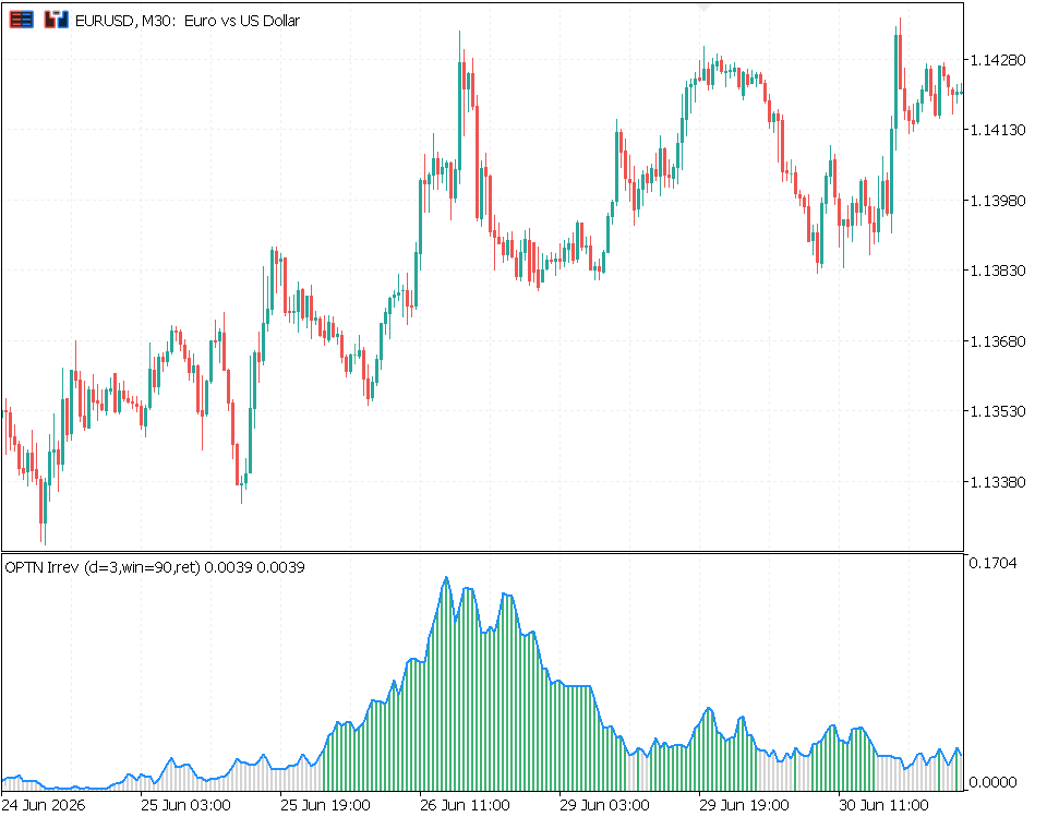
Fig. 4. The regime panel: green histogram columns mark trending stretches, gray marks ranging, with the irreversibility line on top

The efficiency indicator. OPTN_Efficiency computes the permutation entropy per bar, stores it in a rolling history, and plots its percentile rank rather than its raw level. The percentile is computed against past values only, with no look-ahead, by counting how many of the recent stored entropies are less than or equal to the current one:

//+------------------------------------------------------------------+
//| Percentile rank (0..100) of the PE at bar 'idx' within the prior |
//| InpPctLookback stored PE values. Ranks against PAST values only  |
//| (no look-ahead): counts how many recent PEs are <= the current   |
//| one. Returns 50 until enough history has accumulated.            |
//+------------------------------------------------------------------+
double PctRank(const int idx)
  {
   int lo=idx-InpPctLookback;
   if(lo<0)
      lo=0;
   int n=idx-lo;                      // number of prior points available
   if(n<10)
      return 50.0;                    // not enough history yet -> neutral
   double x=g_peHist[idx];
   int c=0;
   for(int j=lo;j<idx;j++)
      if(g_peHist[j]<=x)
         c++;
   return 100.0*(double)c/(double)n;
  }

The calculation loop for this panel requires two steps, implemented in a single pass. It must first know the raw permutation entropy at a bar before it can rank that bar, and the rank needs the entropies of earlier bars, so the indicator maintains a persistent history array, g_peHist, indexed by bar. On each bar it computes the raw entropy, stores it, and then converts it to a percentile against the stored history:

   int start=(prev_calculated>first)?(prev_calculated-1):first;
   double win[];
   for(int i=start;i<rates_total;i++)
     {
      bool onGrid=((i-first)%g_step==0) || (i==rates_total-1);
      double pe=EMPTY_VALUE;
      if(!onGrid && i>first)
        {
         pe=g_peHist[i-1];            // carry prior PE forward between grid points
        }
      else
        {
         int got=BuildWindow(i,win,open,high,low,close);
         if(got>=g_window && g_net.Compute(win,got))
            pe=g_net.PermutationEntropy();
        }

      g_peHist[i]=pe;

      if(pe==EMPTY_VALUE)
        {
         BufPct[i]=EMPTY_VALUE;
         BufRawPE[i]=EMPTY_VALUE;
         continue;
        }
      BufPct[i]  =PctRank(i);
      BufRawPE[i]=InpShowRawPE ? pe*100.0 : EMPTY_VALUE;
     }

The history array is kept the same length as the series and re-initialized whenever the bar count changes, so the percentile is always ranking against genuine prior values, never against uninitialized memory. The panel scales from zero to a hundred with dotted reference levels at twenty and eighty, so an efficiency collapse toward the floor is immediately visible. A raw-entropy line is available as an optional plot for readers who want to see the underlying level, but it is off by default because, as we saw, it barely moves. A dip in the percentile line toward zero is the actionable event: it says the market has just become unusually structured relative to its recent self, which is precisely when the random-walk assumption is weakest.

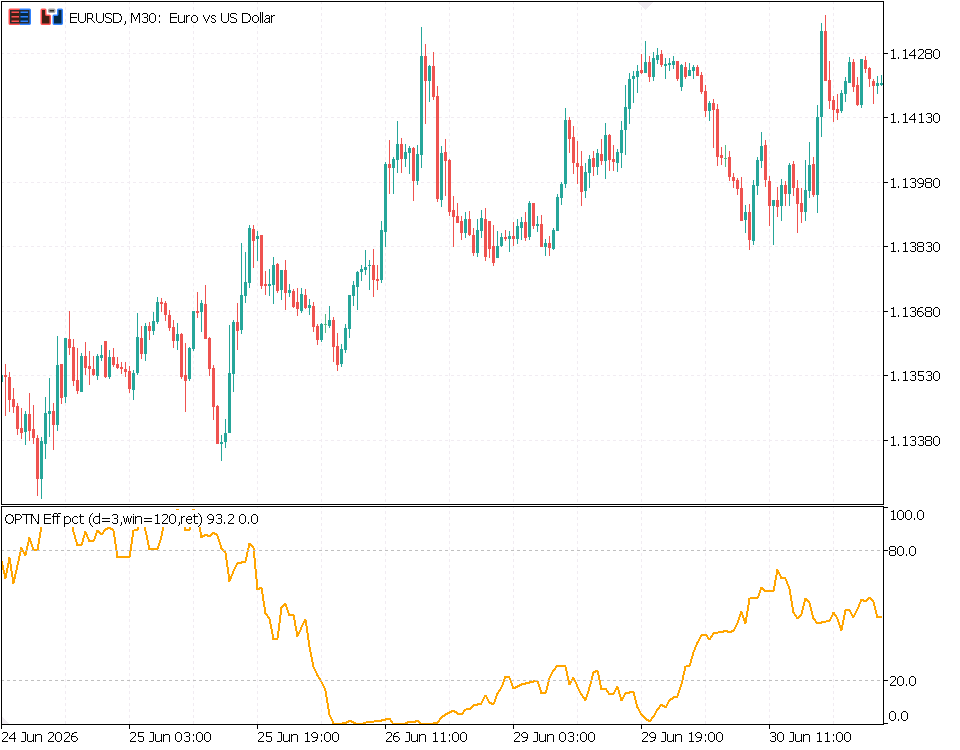
Fig. 5. The efficiency panel: the permutation-entropy percentile dips toward zero when the market becomes unusually structured

Using the two together. The natural reading is to combine them. When the efficiency percentile drops and the regime histogram turns green at the same time, the market has become both structured and directional, the most favorable state for trend-following logic. When efficiency is high and the regime is gray, the series is behaving like an efficient random walk and directional strategies should stand aside. Neither panel is a trade signal on its own; together they are a context filter grounded in the actual complexity of recent price action.

A reference for the shared inputs:

Input	Meaning	Default
InpDimension	Embedding dimension d; alphabet size is d!	3
InpWindowBars	Rolling window per point; clamped up to the engine's minimum	90 (regime), 120 (efficiency)
InpSource	Encode raw price or one-bar log returns	OPTN_RETURN
InpPrice	Base applied price for the transform	PRICE_CLOSE
InpRegimeThresh	Irreversibility level above which the regime is called trending	0.03
InpPctLookback	History length for the entropy percentile rank	250
InpStep	Recompute every N bars and carry forward in between	1

Conclusion

We set out to read the market through shape rather than magnitude, and we built the full pipeline to do it: an ordinal-pattern encoder based on the Lehmer code, a directed transition network over those patterns, and three complexity metrics computed from the network and its time-reversed counterpart. We then turned the two metrics that matter into indicators, a regime panel driven by time-irreversibility and an efficiency panel driven by the percentile of permutation entropy.

• Ordinal patterns are a robust encoding. By keeping only rank order, the method is self-normalizing, noise-tolerant, and comparable across instruments, which sidesteps much of the pain of working with raw price levels.
• Time-irreversibility is the strongest signal here. Comparing the forward and reversed pattern distributions with the Jensen-Shannon divergence gives a bounded, theory-backed way to separate trending from ranging markets.
• Honest tuning beats blind faith. The raw metrics looked dead on EUR/USD until a measured parameter sweep showed that encoding returns over a short window revives irreversibility, and that permutation entropy needs rolling-percentile normalization to be visible on a near-efficient market.
• A reliability-first engine pays off. Explicit status codes, a data-sufficiency floor tied to d!, and guards against flat and degenerate windows keep the tool from producing numbers it cannot support.

The two indicators are complete, self-contained tools. Read together, they form a context filter that tells you when recent price action has become structured and directional, and when it is behaving like an efficient random walk, all from the shape of the last few dozen bars.

The programs presented in this article are intended for educational purposes only. Trading involves substantial risk, and nothing here is financial advice or a guarantee of profit. Always test any tool thoroughly on historical and demo data before considering it for a live account.

Getting the Source Code via MQL5 Algo Forge

All source files are attached to this article below, but the full repository is also available on MQL5 Algo Forge, the community's Git-based platform for sharing and collaborating on trading projects.

File name	Description
MQL5\Include\OPTN\OrdinalNetwork.mqh	Ordinal-pattern transition-network engine: Lehmer encoder, rolling network, permutation entropy, time-irreversibility, forbidden fraction
MQL5\Indicators\OPTN\OPTN_Irreversibility.mq5	Regime panel: time-irreversibility with green/gray trend-versus-range shading
MQL5\Indicators\OPTN\OPTN_Efficiency.mq5	Efficiency panel: permutation entropy rendered as a rolling percentile
MQL5\Scripts\OPTN\OrdinalNetworkTest.mq5	Diagnostic harness: synthetic oracles plus real-data metrics across dimensions and windows
MQL5\Scripts\OPTN\OrdinalNetworkSweep.mq5	Parameter sweep reporting the spread of each metric to find settings that produce a moving signal