Distribution-Free Price Channels in MQL5: Quantile Regression by Iteratively Reweighted Least Squares

Contents

1. Introduction
2. From least squares to quantiles
3. Solving the quantile fit with IRLS
4. Building the channel
5. The channel indicator
6. The width gauge indicator
7. Do the lines really estimate the quantiles?
8. The channel width as a volatility feature
9. Validation in the Strategy Tester
10. Conclusion

Introduction

Almost every price channel a trader draws rests on the same two numbers: a mean and a standard deviation. A regression channel fits a line through the average of the window and offsets its edges by a fixed multiple of the residual standard deviation; a Bollinger band does the same around a moving average. Both inherit an assumption that is rarely stated out loud: that price around its trend is distributed symmetrically, and that a standard deviation is a meaningful description of how far it strays. Real price is neither. Its dispersion is driven by a handful of large bars that inflate the standard deviation, and its excursions above and below the trend are frequently uneven.

In this article we build a channel that makes none of those assumptions. Instead of fitting the mean of the window and measuring a standard deviation, we fit three conditional quantile lines directly: the 0.1, 0.5 and 0.9 quantiles of price as a function of position in the window. Each is fitted independently by minimising a loss function called the pinball loss, using a compact routine called iteratively reweighted least squares (IRLS). The result is a distribution-free channel that never computes a standard deviation, never assumes normality, and is free to be asymmetric where the data is. You will learn how that fit works and how to package it into a reusable class and two MetaTrader 5 indicators. Then we test it: whether the three lines really split the window in the proportions their quantile names promise, how the width compares against the Bollinger width, ATR and regression width on the same lookback, and how a deliberately naive Expert Advisor behaves in the Strategy Tester across four instruments.

From least squares to quantiles

Ordinary least squares (OLS) fits a line by minimising the sum of squared residuals. The line it produces passes through the conditional mean of the data: for any position on the x-axis, the fitted value is the expected value of y there. Squaring the residuals is what pins the fit to the mean, and it is also what makes OLS sensitive to outliers, since a single large residual, once squared, dominates the sum.

Quantile regression replaces the squared residual with a different penalty, one that pins the fit to a chosen quantile rather than the mean. For a target quantile tau (a number between 0 and 1), the penalty applied to a residual r is the pinball loss, also called the check loss:

rho_tau(r) = tau * r if r >= 0, and (tau - 1) * r if r < 0.

The whole method is contained in that asymmetry. A point above the line has a positive residual and is penalised with weight tau; a point below has a negative residual and is penalised with weight (1 - tau). At tau = 0.5 both weights are equal, so minimising the pinball loss minimises the sum of absolute residuals, whose solution is the median. At tau = 0.9 an overshoot costs 0.9 while an undershoot costs only 0.1, so the fit is pulled upward until roughly 90% of the points lie below it. That is exactly the definition of the 0.9 conditional quantile.

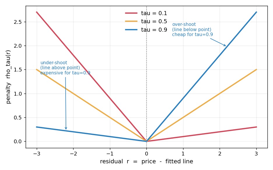
Fig. 1. The pinball loss pins the fit to a chosen quantile: an asymmetric penalty, steep on one side and shallow on the other.

Three properties of this construction matter for a price channel:

• It is distribution-free. No normality is assumed and no standard deviation is ever computed. The quantile is a property of the data itself, whatever its shape.
• It is robust. The loss is linear in the residual, not quadratic, so a single extreme bar cannot dominate the fit.
• The edges are independent. The 0.1 and 0.9 lines are two separate fits. Nothing ties them symmetrically around the median, so the channel can be wider on one side than the other.

The cost of all this is that the pinball loss has no closed-form minimiser the way OLS does. There is no normal-equation formula that hands you the quantile line in one step. That is where IRLS comes in.

Solving the quantile fit with IRLS

The pinball loss is not smooth: it has a kink at r = 0 where its slope jumps from (tau - 1) to tau, visible as the corner at the origin in Fig. 1. A minimiser cannot simply set a derivative to zero, because the derivative is undefined exactly at the points we care about. Iteratively reweighted least squares sidesteps this by turning the awkward loss into a sequence of ordinary weighted least-squares problems, each of which does have a closed-form solution.

The idea is that the pinball loss can be written as a weighted squared residual, if the weight is allowed to depend on the residual. Assign each point its pinball weight (tau above the line, 1 - tau below) divided by the absolute size of its residual. Solve the weighted least-squares line, recompute the residuals against the new line, update the weights, and repeat. Each pass reduces the pinball loss and the line settles. This is a Schlossmacher-type IRLS formulation of quantile regression: Schlossmacher (1973) published the scheme for least absolute deviations, which is the tau = 0.5 case, and the asymmetric weights above generalise it to any tau.

The whole method lives in a single class, CQuantileLine, in QuantileRegression.mqh. It represents one quantile line y = a + b*x, where x is the centred position of a bar inside the window. The constructor clamps tau inside the open interval (0, 1) and stores the controls the IRLS loop needs: an iteration cap, a convergence tolerance, and the epsilon that floors the residual:

//--- construct for a given quantile with sensible IRLS controls
                     CQuantileLine(const double tau = 0.5,
                                   const int maxIter = 200,
                                   const double tol = 1e-6,
                                   const double eps = 1e-6)
     {
      m_tau     = (tau <= 0.0 ? 1e-6 : (tau >= 1.0 ? 1.0 - 1e-6 : tau));
      m_maxIter = (maxIter < 1 ? 1 : maxIter);
      m_tol     = tol;
      m_eps     = eps;
      m_a       = 0.0;
      m_b       = 0.0;
      m_valid   = false;
      m_iters   = 0;
     }

Every IRLS pass calls a weighted least-squares solver: the closed-form solution of a two-by-two normal-equation system, guarded against a singular one.

//--- Weighted least-squares solve of y = a + b*x for the given
//--- per-point weights. Returns false on a degenerate (singular)
//--- normal-equation system, leaving a,b untouched.
   bool              SolveWLS(const double &x[], const double &y[],
                              const double &w[], const int n,
                              double &a, double &b) const
     {
      double sw = 0.0, swx = 0.0, swy = 0.0, swxx = 0.0, swxy = 0.0;
      for(int i = 0; i < n; i++)
        {
         double wi = w[i];
         sw   += wi;
         swx  += wi * x[i];
         swy  += wi * y[i];
         swxx += wi * x[i] * x[i];
         swxy += wi * x[i] * y[i];
        }
      double det = sw * swxx - swx * swx;
      if(MathAbs(det) < 1e-12)
         return(false);
      b = (sw * swxy - swx * swy) / det;
      a = (swy - b * swx) / sw;
      return(true);
     }

With every weight at 1.0 this reduces to ordinary least squares, which is exactly how we seed the iteration. The determinant check returns false rather than dividing by a near-zero number, so a degenerate window such as a run of identical prices fails cleanly instead of producing garbage.

The IRLS loop itself is the Fit method. It seeds from an unweighted fit, then reweights and refits until the coefficients settle or the iteration cap is reached:

//--- fit the quantile line to y[] sampled at centred positions x[].
//--- x[] and y[] must both hold n points; returns true on success.
//--- Convergence is RELATIVE: the movement of the fitted value at the
//--- window edge against its height there, so it is scale-free.
   bool              Fit(const double &x[], const double &y[], const int n)
     {
      m_valid = false;
      m_iters = 0;
      if(n < 2)
         return(false);

      //--- seed from an ordinary (unit-weight) least-squares fit
      double w[];
      ArrayResize(w, n);
      for(int i = 0; i < n; i++)
         w[i] = 1.0;

      double a, b;
      if(!SolveWLS(x, y, w, n, a, b))
         return(false);

      //--- distance from the window centre out to the read-out edge
      double xEdge = MathAbs(x[n - 1]);

      //--- IRLS: reweight by the pinball loss, refit, until settled
      for(int it = 0; it < m_maxIter; it++)
        {
         for(int i = 0; i < n; i++)
           {
            double r = y[i] - (a + b * x[i]);       // signed residual
            //--- pinball weight: tau above the line, 1-tau below,
            //--- divided by |r| so weighted LS mimics the L1-type loss
            double side = (r >= 0.0 ? m_tau : 1.0 - m_tau);
            double ar   = MathAbs(r);
            if(ar < m_eps)
               ar = m_eps;                           // guard the kink at r=0
            w[i] = side / ar;
           }

         double na, nb;
         if(!SolveWLS(x, y, w, n, na, nb))
            return(false);

         //--- edge movement, scored against the line's height there
         double move  = MathAbs(na - a) + MathAbs(nb - b) * xEdge;
         a = na;
         b = nb;
         m_iters = it + 1;
         double scale = MathAbs(a) + MathAbs(b) * xEdge;
         if(scale > 0.0 && move < m_tol * scale)
            break;
        }

      m_a     = a;
      m_b     = b;
      m_valid = true;
      return(true);
     }

Two details are worth pausing on. The if(ar < m_eps) ar = m_eps; line is the guard for the kink: a point that lands exactly on the line has a zero residual, and dividing by it would produce an infinite weight. Flooring the absolute residual at a small epsilon keeps the weight finite and the iteration stable.

The second detail is the convergence test: the obvious stopping rule is wrong. The instinct is to stop when the coefficients stop moving: compute move = |da| + |db| and compare it against a small fixed number. That is what this class did in an earlier revision, with a tolerance of 1e-7, and nothing in the output ever looked amiss.

In practice, that test requires the intercept to change by less than 1e-7 in absolute price units. On EURUSD near 1.10 that is demanding but reachable. On BTCUSD near 20,000 the same constant asks for a relative precision of about 5e-12, which a linearly converging method will not reach in any sane number of passes. The consequence is not a wrong answer but a silent one: the loop ran to its cap on every window, and because the fit was already good long before that, nothing complained. Over BTCUSD daily history, 2,238 of 2,258 windows hit the cap; the same code on EURUSD hit it on 77% of windows instead of 99%, and that gap between two instruments running identical code is the tell.

The fix is to make the test relative. The version above measures how far the fitted value moved at the window edge and scales it by the magnitude of the line there. Both quantities are in price units, so the ratio is dimensionless and means the same thing on every instrument. The edge is the right place to measure because it is the value the indicators read out and plot. With that test in place at a tolerance of 1e-6, a single quantile line settles in a median of roughly 40 to 45 passes, which is why the iteration cap moved from 50 to 200. A channel fits three such lines and is only as converged as its slowest, so the per-channel figures reported later are higher again.

The remaining members are small accessor methods that read the fitted line back out:

//--- fitted value at a centred position x (a + b*x)
   double            ValueAt(const double x) const { return(m_a + m_b * x); }
   double            Intercept()             const { return(m_a); }
   double            Slope()                 const { return(m_b); }
   double            Tau()                   const { return(m_tau); }
   bool              IsValid()               const { return(m_valid); }

//--- IRLS passes the last Fit() used; equals the cap when the
//--- tolerance was never met.
   int               Iterations()            const { return(m_iters);   }
   int               MaxIterations()         const { return(m_maxIter); }

Iterations() is what made that diagnosis possible: without it, a window that converged in twelve passes and one that ran two hundred and gave up are indistinguishable, since both return a plausible line. ValueAt(x) reads the line at any position; because x is centred on the window midpoint, ValueAt(0) returns the value at the centre and the right edge gives the value at the most recent bar.

Building the channel

A single quantile line is only half the story. The channel is three of them, fitted over the same window: the lower quantile, the median, and the upper quantile. The class CQuantileChannel holds three CQuantileLine objects and drives them together. Its constructor takes a single tail probability and maps it to the three taus in the member initialiser list, so a value of 0.1 builds the 0.1 / 0.5 / 0.9 channel: the lower line at tau = 0.1, the median fixed at 0.5, and the upper at 1 - 0.1 = 0.9:

//--- construct the channel for a symmetric quantile pair.
//--- tailProb is the tail mass on each side, so 0.1 gives the
//--- 0.1 / 0.5 / 0.9 channel; the median is always fitted.
                     CQuantileChannel(const double tailProb = 0.1,
                                      const int maxIter = 200) :
                     m_low(tailProb, maxIter),
                     m_mid(0.5, maxIter),
                     m_high(1.0 - tailProb, maxIter)
     {
      m_xRight = 0.0;
      m_valid  = false;
     }

The Fit method builds the x-axis once and passes it to all three lines. Rather than raw bar indices 0, 1, 2 and so on, we centre them on the window midpoint so that x runs from -(n-1)/2 to +(n-1)/2. Centring keeps the numbers small and the normal-equation system well conditioned, and it makes each line's intercept equal to its value at the window centre. The most recent bar sits at x = (n-1) - midpoint, stored as m_xRight for the read-out methods.

//--- fit all three lines to the price window y[0..n-1], where
//--- y[0] is the oldest bar in the window and y[n-1] the newest.
//--- Returns true only if every line fitted successfully.
   bool              Fit(const double &y[], const int n)
     {
      m_valid = false;
      if(n < 2)
         return(false);

      //--- centred x-axis: -(n-1)/2 .. +(n-1)/2, newest bar on the right
      double x[];
      ArrayResize(x, n);
      double mid = (n - 1) / 2.0;
      for(int i = 0; i < n; i++)
         x[i] = i - mid;
      m_xRight = (n - 1) - mid;

      bool ok = m_low.Fit(x, y, n);
      ok = m_mid.Fit(x, y, n) && ok;
      ok = m_high.Fit(x, y, n) && ok;

      m_valid = ok;
      return(ok);
     }

The fit is reported valid only when all three lines succeeded. The read-outs then evaluate each line at the right edge. A second set of ...At(x) accessors evaluates them anywhere inside the window, which is what lets an analysis score every point of a window against its own fitted line rather than only the right edge:

//--- channel read-out at the most recent bar (right window edge)
   double            Lower()  const { return(m_low.ValueAt(m_xRight));  }
   double            Median() const { return(m_mid.ValueAt(m_xRight));  }
   double            Upper()  const { return(m_high.ValueAt(m_xRight)); }

//--- channel read-out at any centred position x inside the window.
//--- x=0 is the window centre, x=m_xRight the most recent bar. Used
//--- to check in-sample coverage across the whole fitted window.
   double            LowerAt(const double x)  const { return(m_low.ValueAt(x));  }
   double            MedianAt(const double x) const { return(m_mid.ValueAt(x));  }
   double            UpperAt(const double x)  const { return(m_high.ValueAt(x)); }

On top of the three levels, the class exposes two derived quantities. The Spread is the vertical distance between the upper and lower lines, a distribution-free measure of how dispersed price is around its trend. The Skew compares the upper half-width (Upper minus Median) against the lower half-width (Median minus Lower), normalised by the total spread, so it lands in the range -1 to +1. Because the two edges are fitted independently, the skew is free to be non-zero: it is positive when the upper half of the channel is the wider one and negative when the downside carries the wider tail. This is a structural property of the construction, not something we impose.

//--- dispersion and asymmetry read-outs at the most recent bar
   double            Spread()   const { return(Upper() - Lower());   }
   double            UpperGap() const { return(Upper() - Median());  }
   double            LowerGap() const { return(Median() - Lower());  }

//--- skew of the channel: >0 when the upper half is the wider one,
//--- <0 when the downside carries the fatter tail. In [-1, +1].
//--- A crossed channel returns 0 here; use Crossed() to tell that
//--- apart from a genuinely symmetric window.
   double            Skew() const
     {
      double s = Spread();
      if(s <= 0.0)
         return(0.0);
      return((UpperGap() - LowerGap()) / s);
     }

That guard on a non-positive Spread is not defensive boilerplate; it is where a real failure mode surfaces. The three lines are fitted independently and nothing requires them to stay in order, so the fitted 0.9 line can end up below the fitted 0.5 line. This is the quantile crossing problem, and it is the price of the independence that gives the channel asymmetry. A symmetric band cannot cross because its edges are offsets from a single centre; ours can, precisely because they are not. It shows up at the window edges, where lines of differing slope have diverged most and where the read-outs are taken. Returning 0 from Skew() keeps the arithmetic safe, but 0 is also what a symmetric channel returns, so that guard alone would convert a broken fit into a plausible reading. The channel therefore exposes the condition directly:

//--- The lines are fitted independently, so they can cross. A crossed
//--- window is a broken fit rather than a signal: sit it out.
   bool              Crossed() const
     {
      return(Lower() > Median() || Median() > Upper());
     }

How often this actually happens is an empirical question rather than a theoretical one, and we measure it later alongside the fitter's other costs. The answer is large enough to matter.

The channel indicator

With the channel logic contained in the include file, the indicator that draws it is thin. QuantileChannel.mq5 declares three plot buffers, one per line, and configures their appearance in the property block at the top of the file. The lower plot is shown here; the median and upper plots repeat the same five properties, with the median at width 2 so it reads as the trend:

#property indicator_chart_window
#property indicator_buffers 3
#property indicator_plots   3

#property indicator_label1  "Lower"
#property indicator_type1   DRAW_LINE
#property indicator_color1  clrTomato
#property indicator_style1  STYLE_SOLID
#property indicator_width1  1

The inputs are the three knobs the reader will turn: the rolling window length, the tail probability that sets the quantile pair, and the applied price. The buffers are plain arrays bound to the plots in OnInit:

input int    InpWindow   = 100;             // Rolling window length (bars)
input double InpTailProb = 0.1;             // Tail probability each side (0.1 -> 0.1/0.5/0.9)
input ENUM_APPLIED_PRICE InpPrice = PRICE_CLOSE; // Applied price

double         LowerBuffer[];               // fitted lower quantile line
double         MedianBuffer[];              // fitted median line
double         UpperBuffer[];               // fitted upper quantile line

OnInit binds the three buffers and sets a short name that echoes the parameters into the data-window header. Its closing lines are the ones worth highlighting: the first InpWindow - 1 bars have no full window behind them, so setting PLOT_EMPTY_VALUE to EMPTY_VALUE leaves them blank rather than drawing a line down to zero, and a window shorter than two bars is rejected outright:

//--- warm-up bars carry no channel yet; keep them off the plot
   PlotIndexSetDouble(0, PLOT_EMPTY_VALUE, EMPTY_VALUE);
   PlotIndexSetDouble(1, PLOT_EMPTY_VALUE, EMPTY_VALUE);
   PlotIndexSetDouble(2, PLOT_EMPTY_VALUE, EMPTY_VALUE);
   return(InpWindow < 2 ? INIT_PARAMETERS_INCORRECT : INIT_SUCCEEDED);

Both indicators pull the price series through the same helper, which maps the chosen applied price to a value per bar. The median, typical, and weighted formulas follow the platform's own definitions:

//+------------------------------------------------------------------+
//| Pull the chosen applied price for bar i into a plain array.      |
//+------------------------------------------------------------------+
double AppliedPrice(const int i,
                    const double &open[], const double &high[],
                    const double &low[], const double &close[])
  {
   switch(InpPrice)
     {
      case PRICE_OPEN:     return(open[i]);
      case PRICE_HIGH:     return(high[i]);
      case PRICE_LOW:      return(low[i]);
      case PRICE_MEDIAN:   return((high[i] + low[i]) / 2.0);
      case PRICE_TYPICAL:  return((high[i] + low[i] + close[i]) / 3.0);
      case PRICE_WEIGHTED: return((high[i] + low[i] + 2.0 * close[i]) / 4.0);
      default:             return(close[i]);
     }
  }

The heart of the indicator is OnCalculate: for each bar that needs it, load the window of InpWindow prices ending at that bar, fit the channel, and store the three levels into the plot buffers. Refitting a full window on every historical bar is not free, so prev_calculated is used to avoid recomputing unchanged bars. On the first call it is 0 and start falls back to the first bar with a full window behind it; on later calls it holds the previous return value, so we resume from the last computed bar. The window is loaded oldest-first to match the centred x-axis inside CQuantileChannel, where index 0 is the oldest bar. A window that fails to fit stores EMPTY_VALUE:

//+------------------------------------------------------------------+
//| Custom indicator iteration function                              |
//+------------------------------------------------------------------+
int OnCalculate(const int rates_total,
                const int prev_calculated,
                const datetime &time[],
                const double &open[],
                const double &high[],
                const double &low[],
                const double &close[],
                const long &tick_volume[],
                const long &volume[],
                const int &spread[])
  {
   if(rates_total < InpWindow)
      return(0);

   CQuantileChannel channel(InpTailProb);
   double win[];
   ArrayResize(win, InpWindow);

//--- only recompute bars that are new since the last call; each bar's
//--- channel is the fit over the InpWindow prices ending at that bar.
   int start = (prev_calculated > InpWindow ? prev_calculated - 1 : InpWindow - 1);
   for(int i = start; i < rates_total; i++)
     {
      //--- load the window ending at bar i (oldest first, newest last)
      for(int k = 0; k < InpWindow; k++)
         win[k] = AppliedPrice(i - InpWindow + 1 + k, open, high, low, close);

      if(channel.Fit(win, InpWindow))
        {
         LowerBuffer[i]  = channel.Lower();
         MedianBuffer[i] = channel.Median();
         UpperBuffer[i]  = channel.Upper();
        }
      else
        {
         LowerBuffer[i]  = EMPTY_VALUE;
         MedianBuffer[i] = EMPTY_VALUE;
         UpperBuffer[i]  = EMPTY_VALUE;
        }
     }
   return(rates_total);
  }

Dropped on a chart, the three lines wrap price directly.

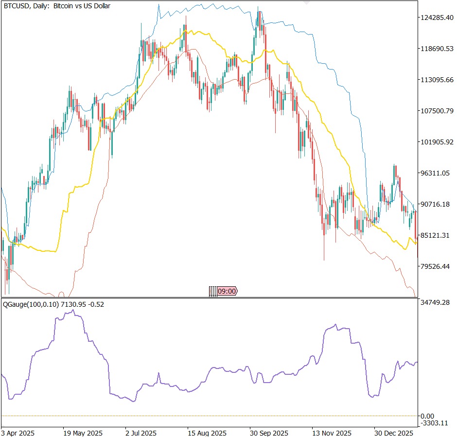
Fig. 2. The quantile channel on the price chart, with the Spread and Skew gauge below.

The width gauge indicator

The second indicator, QuantileChannelGauge.mq5, plots the channel's width and asymmetry in a sub-window instead of on price. It shares the same inputs and the same AppliedPrice helper as the channel indicator, so only its distinguishing parts are shown here. Its property block follows the same shape as the channel's, differing only in declaring indicator_separate_window and two buffers, Spread and Skew, instead of three.

Its OnInit differs in one respect: the Skew oscillates around zero, so a zero reference line is drawn to make its sign readable at a glance.

//--- a zero reference line makes the Skew sign readable at a glance
   IndicatorSetInteger(INDICATOR_LEVELS, 1);
   IndicatorSetDouble(INDICATOR_LEVELVALUE, 0, 0.0);

The calculation loop mirrors the channel's, storing the two derived read-outs instead of the three levels:

if(channel.Fit(win, InpWindow))
        {
         SpreadBuffer[i] = channel.Spread();
         SkewBuffer[i]   = channel.Skew();
        }
      else
        {
         SpreadBuffer[i] = EMPTY_VALUE;
         SkewBuffer[i]   = EMPTY_VALUE;
        }

Do the lines really estimate the quantiles?

Everything so far has been construction. We named three lines after the 0.1, 0.5 and 0.9 conditional quantiles and built machinery that is supposed to produce them, but naming a thing does not make it so. Before asking what the channel is good for, we should ask whether it is what it says it is.

The test is direct. If the upper line really is the 0.9 conditional quantile of price over its window, about 90% of that window's prices should lie below it: not the prices at the right edge, but every price measured against the line at its own position, which is why the class exposes the ...At(x) read-outs. A script, QC_Validation.mq5, slides that count across the history of several instruments and prints the result. Here is the baseline configuration, a 100-bar window at tailProb 0.1, on four instruments from four asset classes:

Instrument	Below lower (target 10%)	Below median (target 50%)	Below upper (target 90%)
BTCUSD D1	10.8%	50.0%	89.2%
EURUSD D1	10.8%	50.0%	89.2%
XAUUSD D1	10.8%	50.0%	89.2%
SPX500 D1	10.8%	50.0%	89.2%

The construction does what it says, and the figures are not merely close to target but identical across four unrelated markets. That is combinatorics rather than coincidence. Quantile regression puts an exact constraint on the answer: the fitted line passes through as many data points as it has parameters, and the fraction of points below it is pinned to within p/n of the target, where p is the number of parameters (an intercept and a slope) and n is the window length. With n = 100 that bound is two percentage points and the count is an integer out of 100, so the achievable values are quantised, whatever the underlying market is doing.

The window sweep confirms the mechanism, because the deviation from target should shrink as the window grows:

Window	Below lower	Deviation from 10%	p/n bound
50 bars	11.7%	1.7 points	4.0%
100 bars	10.8%	0.8 points	2.0%
200 bars	10.4%	0.4 points	1.0%

The deviation halves each time the window doubles, exactly as the bound predicts, and stays comfortably inside it throughout. Changing the tail probability moves the lines to their new targets just as cleanly: at tailProb 0.05 the coverage reads 5.9 / 50.0 / 94.1 against targets of 5 / 50 / 95, and at 0.20 it reads 20.6 / 50.0 / 79.4 against 20 / 50 / 80.

That matters because the IRLS routine here is an approximation. The exact solution to a quantile regression is a linear program, and there was no guarantee in advance that the Schlossmacher iteration would land on the same answer. The coverage test says it does. That is the real content of this section: not that quantile regression estimates quantiles, which is a theorem, but that our implementation of it reproduces the theorem's behaviour on real market data.

The same test, one bar into the future

Everything above is measured in sample: each point is scored against a line fitted using that very point. A trader never gets that; what a trader gets is the channel drawn at the right edge and a bar that has not happened yet. So we run the identical count out of sample, taking the next bar's close against the channel fitted on the window that ended before it:

Instrument	Next bar below lower	Next bar below median	Next bar below upper	Total outside the band
BTCUSD D1	20.9%	45.7%	73.1%	47.8%
EURUSD D1	21.9%	49.7%	79.3%	42.6%
XAUUSD D1	20.4%	49.0%	75.6%	44.8%
SPX500 D1	22.6%	52.4%	74.2%	48.4%

A band whose nominal design leaves 20% of observations outside is leaving between 43% and 48% of next bars outside, on every instrument tested. That is a factor of roughly two and a quarter, and its consistency across markets says it is structural rather than a quirk of one of them.

The reason is not a defect in the fit but the difference between describing and predicting. The channel is an excellent summary of the window it was fitted on. But price is not a stationary draw from that window's distribution: the next bar arrives with its own drift, and the fitted edges are extrapolations to the very boundary of the fitting range, where any linear fit is least reliable. Interpreting the upper line as "price will exceed this only 10% of the time tomorrow" is not supported by the data.

Read the channel as a description, not a forecast. The lines are genuine conditional quantiles of the window they were fitted on, verified to within the theoretical bound on four asset classes. They are not predictive bounds on the next bar: roughly 45% of next bars close outside a band nominally designed to contain 80% of them. Any rule that treats a touch of the upper line as a rare event is mispriced by more than a factor of two.

What the fitter costs

The last part of the audit is the machinery itself: how hard the IRLS loop works, how often it gives up, and how often the independently fitted lines cross each other. All three come from the same run, at the baseline 100-bar window:

Instrument	Windows	Mean IRLS passes (worst of the three lines)	Hit the 200 cap	Failed to fit	Crossed lines
BTCUSD D1	2,265	95.9	13.2%	0	9.1%
EURUSD D1	2,880	78.1	5.6%	0	2.9%
XAUUSD D1	1,590	84.2	8.6%	0	5.4%
SPX500 D1	862	81.0	6.6%	0	7.4%

The mean pass count sits between 78 and 96, an order of magnitude more than the "handful" one might assume, which is why the cap is 200 rather than 50. Between 5.6% and 13.2% of windows still exhaust it; those windows are not wrong, merely not converged to the requested tolerance, and since that tolerance asks for a millionth of the price level the practical difference is far below one tick. The degenerate-system guard in SolveWLS never fired across roughly 7,600 windows.

The crossing figure deserves attention. Between 2.9% and 9.1% of windows produce a channel whose lines are out of order at the right edge, which on BTCUSD is nearly one bar in eleven. Those bars are not a signal and should not be traded or plotted as if the channel were valid, which is why Crossed() exists and why the Expert Advisor sits them out. It is the cost of letting the two edges move independently, and a symmetric Bollinger band never pays it.

The channel width as a volatility feature

The most informative single number this construction produces is the Spread, the distance between the upper and lower lines. There is a mechanical reason to expect it to behave like a volatility measure: the two lines are the 0.9 and 0.1 conditional quantiles of price around its trend, so their gap is a conditional interquantile range, and an interquantile range is a scale estimate. When price disperses widely the lines pull apart; when it settles into a tight drift they close in.

One subtlety has to be handled first. The raw Spread is measured in price units, and Bitcoin's price level ranges over an order of magnitude across this history, so a channel around price at 60,000 has a larger absolute spread than one at 6,000 regardless of how volatile the market is. We therefore compare two things against realised volatility: the raw absolute Spread, and the Spread divided by the current price. Realised volatility is the standard model-free proxy, the standard deviation of the trailing log returns.

The comparison was run over 2,265 daily bars with a 100-bar channel window and a 20-bar realised-volatility lookback:

Comparison	Pearson correlation	Reading
Absolute Spread vs realised volatility	0.010	No relationship: dominated by the price-level trend
Normalised Spread vs realised volatility	0.595	Strong: the width tracks dispersion
Normalised Spread vs forward realised volatility	0.301	Moderate: some leading content

The first row is the control, and it is the reason normalisation matters. The raw absolute Spread has essentially zero correlation with volatility because it is swamped by the long-run rise in price level; anyone reporting a correlation on the absolute width would be measuring the price trend. Normalised by price, the correlation with contemporaneous realised volatility rises to 0.595. The third row looks one step ahead, against the next window's realised volatility: at 0.301 there is some leading information, but the Spread is mainly a contemporaneous measure and we do not claim more.

How complete that collapse is depends on the instrument. Where the price level is comparatively stable the raw width survives, giving 0.450 on EURUSD, 0.530 on XAUUSD and 0.341 on SPX500. Normalisation is therefore not a cosmetic refinement; it is the difference between a working feature and a meaningless one precisely on the instruments where price has trended hardest, which are the ones a volatility feature is most likely to be pointed at.

Standardising the two series and plotting them together makes that 0.595 visible: they rise and fall in step, spike for spike, while staying distinct enough to reflect a correlation well short of one.

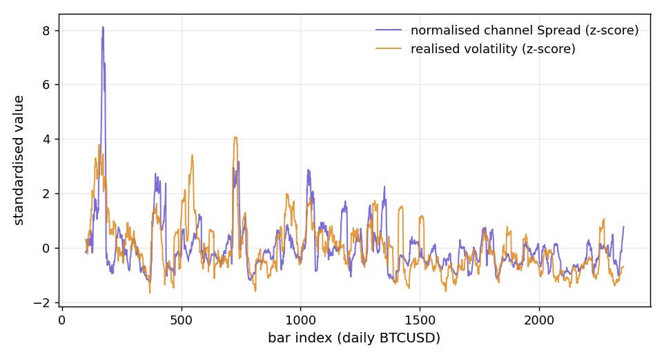
Fig. 3. Normalised channel Spread against realised volatility on daily BTCUSD, both z-scored. Pearson correlation 0.59.

Compared against what?

A correlation of 0.6 sounds respectable in isolation, but "this measures volatility" is a weak claim unless we know what the ordinary tools score on the same data. So we put three alongside: the Bollinger width, the ATR, and the residual width of an ordinary regression channel. One methodological point decides whether the comparison means anything: every measure must see the same lookback. Comparing our 100-bar channel against a conventional ATR(20) on a 20-bar realised-volatility target would have ATR agreeing near 0.9 by construction, since those are two estimators of the same quantity over the same window. Every baseline below is therefore computed over the channel's own 100-bar window.

Instrument	Quantile width	Bollinger width	ATR	Regression width
BTCUSD D1	0.595	0.560	0.404	0.459
EURUSD D1	0.477	0.474	0.694	0.612
XAUUSD D1	0.353	0.672	0.530	0.470
SPX500 D1	0.378	0.153	0.509	0.319

The quantile width is competitive but not superior. It wins on daily Bitcoin, the instrument this article started from, which is exactly the coincidence that produces an over-claiming article if nobody checks the others. Across three timeframes for each of the four instruments, twelve cells in total, the quantile width takes the top spot in two; ATR takes seven and the Bollinger width three, and the regression width never wins anywhere.

That it does not dominate is not a flaw in the implementation. Realised volatility is defined as a standard deviation, so a measure itself built from a standard deviation over the same data starts with a structural advantage in matching it, while our channel is deliberately built to ignore the tails that inflate one. Scoring it against a standard-deviation target asks it to reproduce the very quantity it was designed to be robust to.

Does the effect hold still?

The last thing to check is whether this survives a change of period. There is nothing to optimise here, so a walk-forward in the usual sense does not apply: the channel estimates its lines from the trailing window at every bar and no parameter is ever fitted to the history as a whole. What can be asked is whether the same fixed configuration produces the same relationship in different stretches of time. Splitting each history into three equal, disjoint parts:

Instrument	Full history	First third	Second third	Final third
BTCUSD D1	0.595	0.624	0.414	0.414
EURUSD D1	0.477	0.290	0.541	0.537
XAUUSD D1	0.353	0.078	0.405	0.392
SPX500 D1	0.378	0.099	0.661	0.131

The sign is stable, the magnitude is not. SPX500 swings from 0.099 to 0.661 and back to 0.131 across three consecutive stretches of its own history, and XAUUSD opens at 0.078 before settling near 0.4. Whatever is built on top of this feature should tolerate the coefficient moving by a factor of three.

What this section establishes: the normalised channel width is a genuine volatility feature, positively related to realised volatility on every instrument and timeframe tested. It is not the best such feature: a horizon-matched ATR beats it in seven of twelve cells and the Bollinger width in three, with the quantile width leading in two. Its correlation is also period-dependent, varying by a factor of three or more across thirds of the same history.

All of these figures come from the attached QC_Validation.mq5, which sweeps the symbol list, the timeframes and the parameter axes and prints every table in this section to the log. Run it on your own broker's history and it will print the same tables for your instruments.

Validation in the Strategy Tester

The channel is calibrated in sample, miscalibrated out of sample, and a mid-pack volatility gauge. None of that answers the question a trader asks first: does it carry any tradable information at all? Correlations cannot settle that, so the last part of the article hands the channel to an Expert Advisor and runs it through the Strategy Tester.

The design of that EA matters more than its results. An EA with a stop, a target, a trailing rule and a session filter tells you about the stop, the target, the trailing rule and the session filter; to learn about the channel, everything else has to be stripped out until the channel is the only thing that can be responsible for the outcome. QuantileChannelEA.mq5 is therefore deliberately naive: one position at a time, a fixed lot, no stop, no target, decisions only on closed bars, and not one parameter fitted to the data. Its core is a pair of entry rules that are exact opposites:

//--- the two modes are exact opposites on the same two conditions
   int sig = 0;
   if(px < lower)
      sig = (InpMode == QC_REVERSION ? 1 : -1);
   else
      if(px > upper)
         sig = (InpMode == QC_REVERSION ? -1 : 1);

Mean reversion buys when the close falls below the lower line and sells when it rises above the upper one; breakout does the reverse. That opposition is the point of the test: if the channel locates something real about where price is likely to go next, one of the two directions should be consistently better than the other on more than one instrument. Both modes share a single exit, so the only difference between them is the entry:

//--- one exit for both modes, so only the entry differs between them
   if(dir != 0)
     {
      if((dir > 0 && px >= mid) || (dir < 0 && px <= mid))
        {
         g_pending = 2;
         Execute();
        }
      return;
     }

One more line is where the earlier audit pays off. Before anything else, the EA discards windows whose lines came out in the wrong order:

//--- a crossed channel is a broken fit, not a signal: sit it out
   if(channel.Crossed())
      return;

Without the earlier coverage work we would not have known this affects up to one bar in eleven, and those bars would have been traded as though the channel were meaningful.

All runs below use identical settings: D1 bars from 2015.01.01 to 2026.08.01, window 100, tailProb 0.1, close prices, lot 0.01, deposit 100,000 USD, leverage 1:100, and the tester's 1-minute OHLC model. Nothing was optimised, and no configuration was chosen after seeing its result.

Instrument and mode	Trades	Net profit	Profit factor	Expected payoff	Max drawdown
BTCUSD reversion	59	-1940.66	0.378	-32.89	1.96%
BTCUSD breakout	395	283.33	1.102	0.72	0.21%
EURUSD reversion	112	-265.35	0.738	-2.37	0.34%
EURUSD breakout	687	-405.08	0.758	-0.59	0.51%
XAUUSD reversion	67	-1803.90	0.513	-26.92	1.87%
XAUUSD breakout	334	-2626.10	0.534	-7.86	2.78%
SPX500 reversion	39	-66.91	0.805	-1.72	0.16%
SPX500 breakout	212	-117.93	0.771	-0.56	0.19%

Seven of the eight configurations lose money, and the eighth is not a result. BTCUSD breakout returns 283 currency units on 395 trades, an expected payoff of 0.72 per trade on a 0.01 lot, a profit factor of 1.10 well inside the range that spreads and commissions would erase. More telling is that the pattern does not repeat: if breakout were genuinely the right way to read this channel it should not be losing on the other three instruments, and it loses on all of them. Neither direction wins, which is a clean answer to the question this section was built to ask. The channel edges are not, on their own, a source of entries.

The width as a filter instead of a signal

Since the channel's most informative output is its width rather than its position, the last test gates that same breakout rule on the normalised width, trading only when it is above or below a threshold of 0.20:

BTCUSD breakout with width gate	Trades	Net profit	Profit factor	Expected payoff
No gate	395	283.33	1.102	0.72
Wide channels only	234	-16.65	0.990	-0.07
Narrow channels only	173	531.10	1.589	3.07

Restricting the same rule to narrow channels raises the profit factor from 1.10 to 1.59 while more than halving the trade count, and restricting it to wide channels destroys it. Read at face value that is the most encouraging table in the article, and it is exactly the sort of table that should be distrusted.

Why we do not claim the narrow-width filter works. Ten configurations were tested in this section, and the best of ten draws will look good whether or not anything real is present: 1.589 on 173 trades of a single instrument is not far outside what chance produces at that sample size. Treating it as a finding would require it to reproduce on instruments and periods that were not used to notice it, which is a different experiment from this one.

What can be said without overreaching is that the width behaves like a regime variable rather than a signal. The two gates split the same rule into two clearly different populations, consistent with what the correlation work found. Turning that into a tradable filter is separate work needing its own out-of-sample evidence.

Conclusion

We built a price channel from a different starting point than the usual mean and standard deviation. By fitting conditional quantile lines directly, with the pinball loss solved through an IRLS loop, we obtained a channel that assumes no distribution, resists the influence of individual extreme bars, and is structurally free to be asymmetric. The logic lives in a single reusable include, QuantileRegression.mqh, and two thin indicators put it on the chart: one for the channel itself, one for its width and asymmetry. Four findings came out of testing it:

• The lines are real conditional quantiles. In-sample coverage hits its targets on four asset classes, tracks the theoretical p/n bound as the window grows, and follows the tail probability wherever it is set.
• They are descriptive, not predictive. Out of sample the band leaves more than twice its nominal share of next bars outside it. This is the most likely way to misuse the indicator.
• The width is a genuine but unexceptional volatility feature. Normalised for price level it is positively related to realised volatility everywhere tested, but a horizon-matched ATR beats it more often than not, and its correlation is period-dependent.
• The edges are not a source of entries. A deliberately naive EA trading them lost money in seven of eight configurations, and the two entry rules were exact opposites, so there was no direction left for it to be right about.

Use this channel as an analytical instrument: to see where price sits inside its recent distribution, to read the asymmetry a symmetric band cannot show, and to feed its normalised width into something else as a volatility or regime input. Do not use its edges as entry triggers or read them as probabilistic bounds on the next bar.

Two lessons carry beyond this particular indicator. A convergence tolerance expressed in absolute price units is not portable between instruments, and that kind of bug is invisible: the output stays plausible while the loop quietly never converges. And independently fitted quantile lines can cross, so a construction that permits asymmetry has to be checked for it rather than assumed to behave. Both were found only by measuring, and neither would have shown up on a chart.

File	Type	Description
QuantileRegression.mqh	Include	The CQuantileLine and CQuantileChannel classes: IRLS quantile fitting and the three-line channel with Spread and Skew read-outs.
QuantileChannel.mq5	Indicator	Draws the lower, median and upper quantile lines on the price chart.
QuantileChannelGauge.mq5	Indicator	Plots the channel Spread and Skew in a separate sub-window.
QuantileChannelEA.mq5	Expert Advisor	The deliberately naive tester EA: opposite mean-reversion and breakout entries sharing one median exit, with an optional channel-width regime gate.
QC_Validation.mq5	Script	Reproduces every table in the article: quantile coverage in and out of sample, the horizon-matched width comparison against Bollinger, ATR and regression widths, sub-period stability, and the fitter's iteration, failure and crossing counts.