Measuring the Probability of Backtest Overfitting of Your MetaTrader 5 Optimization (Part 1): The CSCV Engine in MQL5

Contents

• Introduction
• Why the hold-out method is not enough
• The strategies being tested
• The CSCV procedure without the heavy mathematics
• Building the returns matrix
• Making 12,870 splits tractable
• The engine
• Checking the engine before trusting it
• Using it on your own optimization
• The result
• The degradation plot, and why it needs a control
• How much history a sweep really needs
• Limitations
• Conclusion

Introduction

In this article, we measure the Probability of Backtest Overfitting of your MetaTrader 5 optimization. In plain terms, it tells you how likely your optimization process is to have selected noise rather than a real signal.

The measure is the Probability of Backtest Overfitting (PBO) of Bailey, Borwein, López de Prado and Zhu (2015), computed through their Combinatorially Symmetric Cross-Validation (CSCV) procedure. You get one number, and above 5% you reject the optimization procedure and do not trade the strategy it selected. That 5% is the customary cut-off the authors suggest, by analogy with the usual 5% significance level, so it is a convention rather than something the method derives.

This is worth doing every time you optimize. If you run sweeps in the Strategy Tester, you can run the code below on the returns behind them and estimate how likely it is that the retained parameters are due to luck rather than to a structural market effect. Optimizing is not the problem, and optimizing without knowing which of the two you found is.

The method is not mine. My master’s thesis, in quantitative asset and risk management, applied this same framework to a panel of technical indicators on the S&P 500 and the Nasdaq 100, and it is published on SSRN. What is new here is the MetaTrader 5 implementation.

Ignoring backtests that are invalid due to missing costs, financing or bad data, any strategy that beat buy and hold did so for one of two reasons. Either it captured something structural, meaning a recurring pattern in how the market actually works, or it simply lined up with the particular sequence of moves contained in that particular history. The second one is luck, and a backtest cannot tell the two apart, because both produce the same equity curve.

As you test more combinations, the probability that the top result is luck increases. If you test thousands of settings on the same history, a few will look excellent by accident alone, in the same way that a few coins out of a thousand will come up heads ten times in a row. Overfitting, here, does not mean that the code is wrong but that the selection picked the accident.

A structural signal keeps working until whatever produces it goes away, but luck stops working at once, because the next stretch of market is not the one it was fitted to.

Why the hold-out method is not enough

The usual answer to overfitting is the hold-out method. You split the history into two parts, you fit on the first part, and you validate on the second. Those two parts are what everyone calls the in-sample data and the out-of-sample data. If the strategy behaves the same way out-of-sample as it did in-sample, it is considered validated.

It is better than nothing, but it is not enough, and there are three reasons for that.

• The validation half may not be truly out-of-sample. You may never have run a test on it, but the data is public and widely studied, so the strategy ideas you start from could already have been shaped by that same history, consciously or not, and a hold-out cannot tell you whether they were.
• The split itself is a choice. Cut three years off the end and you validate against one regime, cut them off the start and you validate against another, and there is no principled place to cut.
• The third reason settles it: as soon as you test more than one strategy, the best of them is partly selected on noise. The hold-out answers a single yes-or-no question about one strategy, while the sweep in this article runs 1,300 of them, which is thirteen moving average periods times one hundred thresholds.

That last point reframes the problem, because the right question is not whether a backtest is overfitted. Every backtest built by selection is, to some degree, so the question is how much, and that requires a measure rather than a verdict.

The strategies being tested

Two indicators are tested in this article, and the trading rule is the same for both, which is what makes the comparison between them fair.

The MACD on price

It measures the distance between the closing price and its own moving average over n days, expressed as a percentage of that average. If that distance is above the threshold, you go long the S&P 500, and if it is below the threshold, you go short.

A moving average crossover is a picture, and this is the same idea expressed as a number, which is what makes it optimizable. The classic crossover is the special case where this value passes through zero, so testing a range of thresholds means testing the crossover along with everything around it.

Here is the whole indicator. It goes in MQL5\Include\PBO\MACDp.mqh and depends on nothing.

//+------------------------------------------------------------------+
//| Simple moving average of the last n values ending at i.          |
//+------------------------------------------------------------------+
double MacdpSma(const double &price[], const int i, const int n)
  {
   if(n <= 0 || i < n - 1)
      return(0.0);

   double acc = 0.0;
   for(int k = 0; k < n; k++)
      acc += price[i - k];

   return(acc / n);
  }

//+------------------------------------------------------------------+
//| MACD on price over a whole series.                               |
//|                                                                  |
//| price[]    input series, index 0 = oldest                        |
//| n          lookback period of the moving average                 |
//| normalise  true  -> percentage deviation from the average        |
//|            false -> raw distance in price units                  |
//| out[]      output, same size as price[]. The first n-1 values are|
//|            set to EMPTY_VALUE and must be skipped by the caller. |
//|                                                                  |
//| Returns the index of the first valid value, or -1 on error.      |
//+------------------------------------------------------------------+
int MACDPrice(const double &price[], const int n, const bool normalise, double &out[])
  {
   const int size = ArraySize(price);
   if(size <= 0 || n <= 1 || n > size)
      return(-1);

   if(ArrayResize(out, size) != size)
      return(-1);

   for(int i = 0; i < n - 1; i++)
      out[i] = EMPTY_VALUE;

   for(int i = n - 1; i < size; i++)
     {
      const double sma = MacdpSma(price, i, n);

      if(!normalise)
        {
         out[i] = price[i] - sma;
         continue;
        }

      // A flat window cannot happen on real prices, but a zero average
      // would blow up the ratio, so it is guarded rather than trusted.
      out[i] = (sma > 0.0) ? (price[i] - sma) / sma * 100.0 : 0.0;
     }

   return(n - 1);
  }

Bears Power

It measures how far the low of the bar fell below an exponential moving average of the close, which is an average that gives more weight to the recent days. Alexander Elder published it in 1989 as one half of the Elder-Ray indicator, and the more negative the value, the harder the sellers pushed. The rule does not change: above the threshold you are long, below it you are short.

//+------------------------------------------------------------------+
//| Bears Power over a whole series.                                 |
//|                                                                  |
//|   alpha    = 2 / (n + 1)                                         |
//|   EMA_1    = Close_1                                             |
//|   EMA_t    = (Close_t - EMA_{t-1}) * alpha + EMA_{t-1}           |
//|   Bears_t  = Low_t - EMA_t                                       |
//|                                                                  |
//| low[], close[]  input series, index 0 = oldest, same size        |
//| n               period of the exponential moving average         |
//| normalise       true  -> percentage of the average               |
//| out[]           output, first n-1 values set to EMPTY_VALUE so   |
//|                 the exponential average has time to settle       |
//|                                                                  |
//| Returns the index of the first valid value, or -1 on error.      |
//+------------------------------------------------------------------+
int BearsPower(const double &low[], const double &close[], const int n,
               const bool normalise, double &out[])
  {
   const int size = ArraySize(close);
   if(size <= 0 || n <= 1 || n > size || ArraySize(low) != size)
      return(-1);

   if(ArrayResize(out, size) != size)
      return(-1);

   const double alpha = 2.0 / (n + 1.0);

   double ema = close[0];
   for(int i = 0; i < size; i++)
     {
      if(i > 0)
         ema = (close[i] - ema) * alpha + ema;

      if(i < n - 1)                       // warm-up, not reported
        {
         out[i] = EMPTY_VALUE;
         continue;
        }

      if(!normalise)
        {
         out[i] = low[i] - ema;
         continue;
        }

      out[i] = (ema > 0.0) ? (low[i] - ema) / ema * 100.0 : 0.0;
     }

   return(n - 1);
  }

Note the normalise flag in both indicators, because it materially changes what the thresholds mean. Both are built from a subtraction rather than a ratio, so their raw value is expressed in price units. Over fourteen years, the index went from about 1,400 to about 7,800, and a threshold of forty points does not mean the same thing at both ends of that sample. Dividing by the moving average turns the reading into a percentage, which is comparable across the whole period. Without it, the grid would be testing an object that changes nature halfway through.

There is no flat state, so the position is always either long or short. That is why the strategy return is simply the market return, with its sign flipped whenever the position is short, and it means the strategy carries the same absolute exposure as holding the index on every bar. Its standard deviation can still differ slightly from that of the market, because flipping the sign on some days changes the average return, but on this data the two stay within about 0.1% of each other for every one of the 1,300 combinations. Any outperformance therefore comes from timing alone rather than from taking more risk.

Two parameters, and where the 1,300 comes from

Each strategy has exactly two numbers to optimize.

• The period, which is the number of days used to compute the moving average. It is tested from 2 to 14, so 13 values.
• The level, which is the threshold the indicator is compared to. It is tested at 100 values, spread across the range the indicator actually reaches on this market at the longest period.

Every pair of those two numbers is one strategy, so 13 periods multiplied by 100 levels gives 1,300 combinations. That is the number the sweep has to choose from, and it is the N used everywhere below.

The CSCV procedure without the heavy mathematics

A CSCV procedure is simply this. You take the whole set of data, you cut it into a fixed number of blocks, sixteen in our case, and then you form every possible way of splitting those blocks into two halves. One half trains, the other half tests, and you do it again for the next combination. Instead of one arbitrary split, you use all of them.

With sixteen blocks taken eight at a time, there are 12,870 such splits, and the testing half is always exactly the blocks the training half did not take.

For each of those splits, you do what you would do in real life, which is to find the parameter combination that performed best on the training half. Then you look at where that same combination ranks on the testing half, among all 1,300 combinations. If the selection carries real information, the combination should rank near the top out-of-sample, and if it was picking noise, its rank is a coin toss.

That relative rank, written as a fraction between zero and one, is called omega, and the paper turns it into a number called a logit, written lambda:

lambda = ln( omega / (1 - omega) )

The logit comes out positive when the rank sits above the middle of the 1,300 and negative when it sits below, so the Probability of Backtest Overfitting is the share of the 12,870 splits whose logit came out at or below zero. Said without any of that vocabulary: it is how often the combination you would have picked in real life ended up in the bottom half of the pack on the data it had not seen.

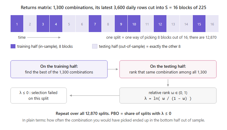
One design detail is important and easy to overlook. The rows are never shuffled, so each block is a run of consecutive bars and keeps the serial dependence and the market conditions of its own period, which a k-fold with shuffled rows would destroy. The blocks themselves are recombined regardless of their dates, however, so in all but one of the 12,870 splits the training half contains at least one block that comes after a testing block. CSCV therefore measures how consistently the selection holds up across different periods of the same history, and it is not a walk-forward test of what would have come next.

Building the returns matrix

The matrix is the only input the engine needs, and building it correctly is most of the work. One column per parameter combination, one row per bar. The loop that fills it is short, since the position is always either long or short, and the care goes into the three details that follow it.

//--- the first usable bar is the one where every period already has a
//--- valid reading on the PREVIOUS bar, so the whole grid shares the
//--- same rows and the matrix stays rectangular
const int first = InpPeriodMax;
const int T     = bars - first;

double market[];                              // log return of the index
ArrayResize(market, T);
for(int t = 0; t < T; t++)
  {
   const int b = first + t;
   market[t] = MathLog(close[b] / close[b-1]);
  }

The indicator is computed once per period rather than once per combination, because it does not depend on the threshold. That is the difference between 13 indicator passes and 1,300 of them.

double ind[];                                 // nPeriods x bars
ArrayResize(ind, nPeriods * bars);

for(int p = 0; p < nPeriods; p++)
  {
   double one[];
   const int n  = InpPeriodMin + p;
   const int ok = (InpIndicator == PBO_IND_MACDP)
                  ? MACDPrice(close, n, InpNormalise, one)
                  : BearsPower(low, close, n, InpNormalise, one);

   if(ok < 0)
     {
      PrintFormat("%s failed for period %d", indName, n);
      return;
     }
   for(int i = 0; i < bars; i++)
      ind[p * bars + i] = one[i];
  }

Then every column is filled by comparing that series to its threshold. The signals counter is not decoration, since it is what lets you find out later whether the winning combination is a real strategy or a column that never changes position.

// Note: "matrix" is a reserved type name in MQL5, hence retMatrix.
double retMatrix[];
if(ArrayResize(retMatrix, T * N) != T * N)
  {
   Print("Cannot allocate the returns matrix.");
   return;
  }

int signals[];                                // position changes per column
ArrayResize(signals, N);
ArrayInitialize(signals, 0);

for(int p = 0; p < nPeriods; p++)
  {
   for(int l = 0; l < nLevels; l++)
     {
      const int    n     = p * nLevels + l;   // column index
      const double level = lo + l * step;

      int prevSign = 0;
      for(int t = 0; t < T; t++)
        {
         const int    b   = first + t;
         const double val = ind[p * bars + (b - 1)];   // signal on the closed bar
         const int    s   = (val > level) ? 1 : -1;

         if(prevSign != 0 && s != prevSign)
            signals[n]++;
         prevSign = s;

         retMatrix[t * N + n] = s * market[t];
        }
     }
  }

Three details in those lines decide whether the result means anything.

• Log returns, not simple returns. A log return is the logarithm of the ratio between two closes, and the property that matters here is that the log returns of several days add up to the return of the whole stretch, which is not true of percentage returns. The whole engine rests on that, and with simple returns it will not fail loudly but will return wrong numbers quietly.
• The signal is read on the previous bar, b - 1 and not b. Reading it on the current bar would use a value that did not exist yet when the position was taken.
• The variable is not called matrix, because in modern MQL5 matrix and vector are built-in types. The compiler answers “unexpected token” without explaining why.

The threshold range is read from the data

A grid needs bounds, and hard-coding them is where most parameter sweeps quietly go wrong, because a range that suits one instrument is meaningless on another.

Instead, the range is derived from the observed distribution of the indicator. Compute it on the longest period tested, sort the values, and take the first and ninety-ninth percentiles, which keeps the extremes the market actually reaches and drops the few extreme readings that would stretch the grid over empty space.

//+------------------------------------------------------------------+
//| Percentile of an already sorted array, nearest rank.             |
//+------------------------------------------------------------------+
double PercentileSorted(const double &sorted[], const double pct)
  {
   const int n = ArraySize(sorted);
   if(n == 0) return(0.0);

   int idx = (int)MathRound(pct / 100.0 * (n - 1));
   if(idx < 0)      idx = 0;
   if(idx > n - 1)  idx = n - 1;
   return(sorted[idx]);
  }

//--- collect the readings of the longest period, ignoring the warm-up
double sample[];
ArrayResize(sample, 0);
for(int i = InpPeriodMax - 1; i < bars; i++)
  {
   const double v = ind[(nPeriods - 1) * bars + i];
   if(v == EMPTY_VALUE) continue;
   const int k = ArraySize(sample);
   ArrayResize(sample, k + 1);
   sample[k] = v;
  }
ArraySort(sample);

const double lo = PercentileSorted(sample, InpTrimPct);
const double hi = PercentileSorted(sample, 100.0 - InpTrimPct);

if(hi <= lo)
  {
   Print("Degenerate threshold range.");
   return;
  }

const double step = (hi - lo) / (nLevels - 1);
PrintFormat("Threshold range from data: %.4f to %.4f in %d steps of %.4f%s",
            lo, hi, nLevels, step, InpNormalise ? " (percent)" : "");

On this data, that returned a range of -5.50% to +4.21% for the MACD on price, and -6.15% to +2.25% for Bears Power. Neither would have been guessed correctly by hand.

Making 12,870 splits tractable

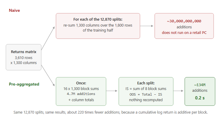
The naive procedure recomputes the 1,300 combinations over the 1,800 rows of a training half for each of the 12,870 splits, which comes to about 30 billion operations and is impractical on a typical retail machine. Sixteen blocks of 225 rows cover 3,600 of the 3,610 rows in the matrix, so the engine drops the 10 oldest, as the comment in the code below says, and a half is eight of those blocks.

Two observations collapse those 30 billion operations. The first is that a cumulative log return is additive, so instead of touching rows you pre-aggregate once into an S by N matrix holding the sum for each block and each combination. A split’s training value is then a sum of eight numbers rather than 1,800.

//+------------------------------------------------------------------+
//| Pre-aggregation: S x N partition sums, plus the column totals.   |
//|                                                                  |
//| Rows are NOT shuffled. Each partition is a contiguous run of     |
//| bars, so serial dependence and seasonal effects survive inside   |
//| it, while the partitions themselves are combined in any order.   |
//|                                                                  |
//| If T is not divisible by S the remainder is dropped from the     |
//| OLDEST end, keeping the most recent history intact.              |
//+------------------------------------------------------------------+
bool CCSCVEngine::Aggregate(void)
  {
   const int S       = m_partitions;
   const int N       = m_cols;
   const int perPart = m_rows / S;

   if(perPart < 1)
     {
      Print("CSCV: ", m_rows, " rows cannot be split into ", S, " partitions");
      return(false);
     }

   const int offset  = m_rows - perPart * S;   // dropped oldest rows
   if(offset > 0)
      PrintFormat("CSCV: dropping %d oldest row(s) so %d rows split evenly into %d partitions",
                  offset, perPart * S, S);

   if(ArrayResize(m_part, S * N) != S * N)
      return(false);
   if(ArrayResize(m_total, N) != N)
      return(false);

   ArrayInitialize(m_part,  0.0);
   ArrayInitialize(m_total, 0.0);

   for(int s = 0; s < S; s++)
     {
      const int base    = s * N;
      const int rowFrom = offset + s * perPart;
      const int rowTo   = rowFrom + perPart;

      for(int t = rowFrom; t < rowTo; t++)
        {
         const int rBase = t * N;
         for(int n = 0; n < N; n++)
            m_part[base + n] += m_returns[rBase + n];
        }
     }

   for(int s = 0; s < S; s++)
     {
      const int base = s * N;
      for(int n = 0; n < N; n++)
         m_total[n] += m_part[base + n];
     }

   return(true);
  }

The second observation is that the testing half is the exact complement of the training half, which means:

OOS = Total - IS

The out-of-sample side is never computed at all, since it is one subtraction. Cost drops to about 134 million additions, plus about 67 million simple operations that the naive procedure needs as well, to reset the sums, find the best in-sample value and count the rank. The measured time for the full 12,870 splits on the 3,610 by 1,300 matrix is 0.2 seconds. The same approach extends to the Sharpe ratio, because the sum, the sum of squares and the count are additive at the block level. For the strategies in this article, the Sharpe ratio would select exactly the same combinations and give the same PBO, because a position that is always one unit long or short has the same sum of squared returns in every column, so the two measures rank the columns in the same order.

The engine

The class is deliberately narrow, since it takes a returns matrix and gives back a number and two distributions, and it knows nothing about symbols, indicators or trading. That is what makes it reusable on a sweep that has nothing to do with the one in this article.

//+------------------------------------------------------------------+
//| CCSCVEngine                                                      |
//+------------------------------------------------------------------+
class CCSCVEngine
  {
private:
   //--- input
   int      m_rows;              // T, number of bars
   int      m_cols;              // N, number of parameter combinations
   int      m_partitions;        // S, must be even
   double   m_returns[];         // T x N log returns, row-major: [t * N + n]

   //--- pre-aggregation
   double   m_part[];            // S x N partition sums, row-major: [s * N + n]
   double   m_total[];           // N total sums

   //--- results, one entry per combination
   double   m_logits[];
   double   m_selIS[];           // IS cumulative log return of the selected trial
   double   m_selOOS[];          // OOS cumulative log return of the selected trial
   int      m_selIndex[];        // which trial was selected

   int      m_combinations;
   double   m_pbo;
   double   m_probLoss;
   bool     m_ready;

   bool     Aggregate(void);
   bool     Enumerate(void);

public:
            CCSCVEngine(void);

   //--- setup
   bool     SetReturns(const double &data[], const int rows, const int cols);
   bool     SetPartitions(const int s);

   //--- run
   bool     Run(void);

   //--- results
   bool     IsReady(void)           const { return(m_ready);          }
   double   PBO(void)               const { return(m_pbo);            }
   double   ProbabilityOfLoss(void) const { return(m_probLoss);       }
   int      CombinationCount(void)  const { return(m_combinations);   }
   int      Rows(void)              const { return(m_rows);           }
   int      Cols(void)              const { return(m_cols);           }

   bool     GetLogits(double &out[]) const;
   bool     GetDegradation(double &is[], double &oos[]) const;
   bool     GetSelected(int &out[])  const;

   //--- control experiment
   bool     RunControl(const int &pool[], const int seed,
                       double &outIS[], double &outOOS[]);
  };

GetSelected is not in the original paper. It returns which combination was chosen on each of the 12,870 splits, and it turns out to be the most informative output of the whole engine.

The 12,870 splits are enumerated as 16-bit masks with exactly eight bits set, which yields the expected count.

//+------------------------------------------------------------------+
//| Number of set bits. Kernighan's loop: v & (v-1) clears the       |
//| lowest set bit, so this runs once per bit actually set.          |
//+------------------------------------------------------------------+
int PopCount(uint v)
  {
   int c = 0;
   while(v)
     {
      v &= (v - 1);
      c++;
     }
   return(c);
  }

Enumerate is the whole procedure in one function. Read it once through, since everything the article has described so far is in it: the pre-aggregated training sum, the best in-sample trial, the complement, the rank and the logit.

//+------------------------------------------------------------------+
//| Walk every combination of S/2 partitions out of S.               |
//|                                                                  |
//| For each: build the training set, take the best trial in sample, |
//| find where that same trial ranks out of sample, and turn the     |
//| relative rank into a logit. Logits at or below zero are the      |
//| failures the PBO counts.                                         |
//+------------------------------------------------------------------+
bool CCSCVEngine::Enumerate(void)
  {
   const int  S    = m_partitions;
   const int  N    = m_cols;
   const int  half = S / 2;
   const uint end  = (uint)1 << S;

   double is[];
   if(ArrayResize(is, N) != N)
      return(false);

   //--- C(S, S/2); allocate generously, we trim at the end
   int cap = 1;
   for(int i = 0; i < half; i++)
      cap = (int)((double)cap * (S - i) / (i + 1));

   if(ArrayResize(m_logits,   cap) != cap) return(false);
   if(ArrayResize(m_selIS,    cap) != cap) return(false);
   if(ArrayResize(m_selOOS,   cap) != cap) return(false);
   if(ArrayResize(m_selIndex, cap) != cap) return(false);

   int          c        = 0;
   int          failures = 0;
   int          losses   = 0;
   const double denom    = (double)(N + 1);

   for(uint mask = 0; mask < end; mask++)
     {
      if(PopCount(mask) != half)
         continue;

      //--- training set: sum the chosen partitions
      ArrayInitialize(is, 0.0);
      for(int s = 0; s < S; s++)
        {
         if((mask & ((uint)1 << s)) == 0)
            continue;

         const int base = s * N;
         for(int n = 0; n < N; n++)
            is[n] += m_part[base + n];
        }

      //--- best trial in sample
      int    bestN  = 0;
      double bestIS = is[0];
      for(int n = 1; n < N; n++)
        {
         if(is[n] > bestIS)
           {
            bestIS = is[n];
            bestN  = n;
           }
        }

      //--- its out-of-sample value, by complement
      const double bestOOS = m_total[bestN] - bestIS;

      //--- rank of that value among all trials out of sample
      int below = 0;
      for(int n = 0; n < N; n++)
        {
         if((m_total[n] - is[n]) < bestOOS)
            below++;
        }

      const double rank  = (double)(below + 1);
      const double omega = rank / denom;                 // strictly inside (0,1)
      const double logit = MathLog(omega / (1.0 - omega));

      m_logits[c]   = logit;
      m_selIS[c]    = bestIS;
      m_selOOS[c]   = bestOOS;
      m_selIndex[c] = bestN;

      if(logit <= 0.0)
         failures++;
      if(bestOOS < 0.0)
         losses++;

      c++;
     }

   m_combinations = c;
   ArrayResize(m_logits,   c);
   ArrayResize(m_selIS,    c);
   ArrayResize(m_selOOS,   c);
   ArrayResize(m_selIndex, c);

   if(c == 0)
      return(false);

   m_pbo      = 100.0 * (double)failures / (double)c;
   m_probLoss = 100.0 * (double)losses   / (double)c;

   return(true);
  }

Finding the rank does not need a sort, since counting how many combinations scored strictly below the selected one is a single pass, which is cheaper. Ties are settled by two fixed rules. A combination equal to the selected one out-of-sample is not counted below it, which puts the selected one at the bottom of its group and errs on the side of a higher PBO. A tie for the best in-sample value goes to the first combination in column order, because the search above only replaces the leader when it finds a strictly higher value. And dividing by N + 1 rather than N means the fraction can never come out at exactly zero or exactly one, which matters because the logarithm of zero has no value and the calculation would fail when the selected combination ranks first or last.

The public entry point is thin, and it times itself so you can see how long the run takes.

//+------------------------------------------------------------------+
//| Run the full procedure.                                          |
//+------------------------------------------------------------------+
bool CCSCVEngine::Run(void)
  {
   m_ready = false;

   if(m_rows == 0 || m_cols == 0)
     {
      Print("CSCV: no returns matrix loaded");
      return(false);
     }

   const uint t0 = GetTickCount();

   if(!Aggregate())
      return(false);
   if(!Enumerate())
      return(false);

   m_ready = true;

   PrintFormat("CSCV: %d combinations over %d trials, %d bars, %d partitions in %.1f s",
               m_combinations, m_cols, m_rows, m_partitions,
               (GetTickCount() - t0) / 1000.0);
   PrintFormat("CSCV: PBO = %.2f%%   Probability of loss = %.2f%%",
               m_pbo, m_probLoss);

   return(true);
  }

The full file is about 500 lines and is published on MQL5 Algo Forge. Download CSCVEngine.mqh, place it in MQL5\Include\PBO\ and use it as is, since it depends only on the standard library.

Checking the engine before trusting it

An engine that has not been checked against known answers cannot be used to check anything else, so before running it on real data it is run on two cases whose answer is fixed in advance.

The first is pure noise, meaning 200 columns of independent random returns with no skill anywhere. The in-sample winner is then a coin toss out-of-sample, so the PBO must come out near 50% on average.

The second plants one genuinely superior column, present in every block. The selection must find it every time, so the PBO must be zero, and since that column always ranks first out of 200 its logit must equal ln(200) exactly on every split.

#include <PBO/CSCVEngine.mqh>

input int InpRows       = 1600;   // bars
input int InpCols       = 200;    // parameter combinations
input int InpPartitions = 16;     // S
input int InpSeed       = 20260815;

//+------------------------------------------------------------------+
//| Standard normal deviate, Box-Muller. MathRand is seeded by the   |
//| caller so the whole test is reproducible.                        |
//+------------------------------------------------------------------+
double Gauss(void)
  {
   double u1 = (MathRand() + 1.0) / 32768.0;   // (0,1], never exactly 0
   double u2 = (MathRand() + 0.5) / 32768.0;
   return(MathSqrt(-2.0 * MathLog(u1)) * MathCos(2.0 * M_PI * u2));
  }

//+------------------------------------------------------------------+
//| Mean and standard deviation of an array.                         |
//+------------------------------------------------------------------+
void MeanSd(const double &v[], double &mean, double &sd)
  {
   const int n = ArraySize(v);
   mean = 0.0; sd = 0.0;
   if(n < 2) return;

   for(int i = 0; i < n; i++) mean += v[i];
   mean /= n;

   for(int i = 0; i < n; i++) { const double d = v[i] - mean; sd += d * d; }
   sd = MathSqrt(sd / (n - 1));
  }

//+------------------------------------------------------------------+
//| Fill a T x N matrix of log returns.                              |
//|                                                                  |
//| edge > 0 gives column `star` a constant per-bar drift, which     |
//| makes it dominate in every partition.                            |
//+------------------------------------------------------------------+
void BuildMatrix(double &m[], const int rows, const int cols,
                 const double edge, const int star)
  {
   const double vol = 0.01;

   for(int t = 0; t < rows; t++)
     {
      const int base = t * cols;
      for(int n = 0; n < cols; n++)
         m[base + n] = vol * Gauss() + ((n == star) ? edge : 0.0);
     }
  }

//+------------------------------------------------------------------+
//| Run one case and report.                                         |
//+------------------------------------------------------------------+
void RunCase(const string label, const double edge, const int star,
             const double pboLow, const double pboHigh)
  {
   double m[];
   if(ArrayResize(m, InpRows * InpCols) != InpRows * InpCols)
     {
      Print("cannot allocate matrix");
      return;
     }

   MathSrand(InpSeed);
   BuildMatrix(m, InpRows, InpCols, edge, star);

   CCSCVEngine engine;
   if(!engine.SetPartitions(InpPartitions)) return;
   if(!engine.SetReturns(m, InpRows, InpCols)) return;
   if(!engine.Run()) return;

   double logits[];
   engine.GetLogits(logits);

   double mean, sd;
   MeanSd(logits, mean, sd);

   const double pbo    = engine.PBO();
   const bool   passed = (pbo >= pboLow && pbo <= pboHigh);

   PrintFormat("--- %s", label);
   PrintFormat("    PBO              = %6.2f%%   (expected %.0f%% to %.0f%%)  %s",
               pbo, pboLow, pboHigh, passed ? "PASS" : "FAIL");
   PrintFormat("    probability of loss = %6.2f%%", engine.ProbabilityOfLoss());
   PrintFormat("    logits: mean %+.3f, sd %.3f, count %d",
               mean, sd, engine.CombinationCount());
  }

//+------------------------------------------------------------------+
//| Script entry point                                               |
//+------------------------------------------------------------------+
void OnStart(void)
  {
   PrintFormat("CSCV validation: %d bars, %d trials, S = %d, seed %d",
               InpRows, InpCols, InpPartitions, InpSeed);

   // No skill anywhere. The in-sample winner is a coin toss out of sample,
   // so roughly half the combinations should land below the median.
   RunCase("CASE A - pure noise", 0.0, -1, 40.0, 60.0);

   // One strategy is genuinely better, in every partition.
   // The engine must recognise it and report almost no overfitting.
   RunCase("CASE B - one persistent winner", 0.004, 7, 0.0, 2.0);

   Print("--- done. Case A near 50% and case B near 0% means the arithmetic holds.");
  }

Both pass. Pure noise returned 43.9%, 44.8% and 54.3% on three different seeds, straddling 50% as it should, but one noise run is only a loose check, because the 12,870 splits all reuse the same sixteen blocks. Over seeds 1 to 2,000, the noise case averages 50.8%, yet only about half of the runs land inside the 40% to 60% band the script checks, so a run outside it is not by itself a sign of a bug. The planted winner returned 0.00% with a logit standard deviation of zero and a mean of 5.298 on every seed, which is ln(200) to four decimals.

The second case proves the ranking and the logit arithmetic exactly, rather than merely making them look plausible, which is why the test file carries both and not just the first one. The file checks only those two ends, and only at one size unless its inputs are changed, so it does not cover a weak edge, columns that are duplicated, mirrored or never trade, or other values of S, N and T.

While running it, one detail in the original paper turns out to be loose. Bailey and his co-authors write that under no information the logits approximate the standard Normal distribution with a standard deviation of 1. If relative ranks are uniform, the logit follows a standard logistic distribution, whose standard deviation is pi over the square root of three, so 1.814 and not 1. One run gives only a rough estimate of that standard deviation, because it moves a lot from one seed to the next, from 1.697 on one seed to 2.388 on the default one. Pooled over seeds 1 to 2,000, it comes out at 1.750, against 1.746 for uniform ranks over 200 strategies, which is what the logistic distribution predicts and not what the Normal one in the paper does.

Using it on your own optimization

The engine needs one thing from you, which is a matrix holding the return of every parameter set on every bar. That is the part MetaTrader does not give you, because the Strategy Tester reports one summary line per pass and not the bar-by-bar series behind it. You have to produce the series yourself, and the loop below is the whole pattern.

#include <PBO/CSCVEngine.mqh>

// bars : number of rows you will use
// sets : number of parameter combinations you are testing
double retMatrix[];
ArrayResize(retMatrix, bars * sets);

for(int n = 0; n < sets; n++)                 // your parameter sets
  {
   ApplyYourParameters(n);                    // whatever configures your strategy
   for(int t = 0; t < bars; t++)
      retMatrix[t * sets + n] = YourStrategyLogReturnOnBar(t);
  }

CCSCVEngine engine;
engine.SetPartitions(16);
if(!engine.SetReturns(retMatrix, bars, sets))
   return;
if(!engine.Run())
   return;

PrintFormat("PBO = %.2f%%", engine.PBO());

//--- which parameter set was chosen, and how often
int sel[];
engine.GetSelected(sel);

int hits[];
ArrayResize(hits, sets);
ArrayInitialize(hits, 0);
for(int i = 0; i < ArraySize(sel); i++)
   hits[sel[i]]++;

Two constraints carry over. The returns must be logarithmic, because the whole engine rests on them being additive, and the signal that decides the position on bar t must be read on bar t - 1.

If your strategy opens and closes positions rather than holding a signed exposure, the return on a bar is simply the change in equity over that bar, expressed as a log return of the account. The engine does not care where the numbers came from, only that the same convention is used in every column.

The result

The setup is an IC Markets demo account, S&P 500 CFD, daily, from 6 August 2012 to 14 August 2026, which is 3,624 bars. The grid is the 1,300 combinations described earlier, and S is 16. Buy and hold returned 454% over the 3,610 rows of the returns matrix, which start once the 14-day average has its first reading, and 443% over the 3,600 rows the engine splits into blocks. On a half, meaning any eight of the sixteen blocks, it returned anywhere from 39% to 292% depending on which eight, so every comparison below uses buy and hold over the same half the strategy was tested on.

Note the broker, because a CFD is not an index. Depth of history, closing times and prices all vary from one broker to the next, so your own run will not reproduce these numbers to the decimal. Press Home on your own daily chart before assuming you have the same starting point, and set the maximum bars in chart to unlimited in Tools > Options > Charts, or you will read a truncated history.

PBO run on US500 D1   |   MACD on price, normalised
3624 bars, 2012.08.06 to 2026.08.14
Threshold range from data: -5.5023 to 4.2062 in 100 steps of 0.0981 (percent)
Grid: periods 2..14 x 100 levels = 1300 combinations
Matrix: 3610 rows x 1300 columns (35.8 MB)
Buy and hold over the period: 454.4% cumulative
CSCV: dropping 10 oldest row(s) so 3600 rows split evenly into 16 partitions
CSCV: 12870 combinations over 1300 trials, 3610 bars, 16 partitions in 0.2 s
CSCV: PBO = 6.99%   Probability of loss = 2.36%
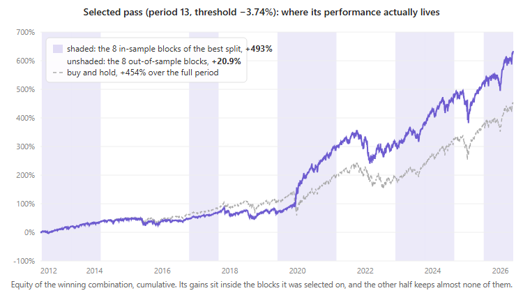
Best in-sample half seen across all splits: 493.0% cumulative
Same parameters out of sample on that split: 20.9%
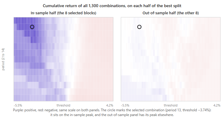
That winner is period 13, threshold -3.737, 64 position changes
Columns ever selected: 84 out of 1300
Near degenerate columns (fewer than 10 changes): 79 of 1300 (6.1%)
Logits: mean +0.906, sd 0.620 over 12870 splits

A PBO of 6.99% fails, since the conventional threshold is 5%. The number printed beside it, the probability of loss, is the share of splits where the combination chosen in-sample went on to lose money out-of-sample, and at 2.36% it is low, which is what you would expect on an index that rose over the period.

The two numbers to look at first are in the middle of that block. The best in-sample half returned 493% cumulative, and the same parameters applied to the other half returned 20.9%, while doing nothing at all over that same half returned 44.1%. That split is one of the dozen splits where the index itself rose most over the training half, by 277%, which is where the winning combination, long 97% of the time, gets its best backtest, and it leaves one of the weakest halves of the 12,870 for testing.

Three checks stand between that number and accepting it, and they are the reason GetSelected exists. Only 6.1% of the grid is near-degenerate, all of it on periods 2 to 5, which passes this check only in part, because almost a quarter of the columns change position fewer than 30 times and stay close to permanently long or permanently short. The winning combination makes 64 position changes over 3,610 bars, so although it is long 97% of the time it acts on its signal rather than being a permanently long column in disguise. And only 84 of the 1,300 combinations are ever chosen, with the top five taking 52.7%, so the procedure concentrates rather than picking at random.

A sane and concentrated selection procedure therefore still fails the test, although 6.99% is close enough to 5% that the way the grid is built and charging trading costs can each move it to the other side, as the Limitations section shows.

The threshold on the winning combination is negative, so the strategy is long by default and flips short only when price falls more than 3.7% below its 13-day average, which makes it a crash avoidance rule. On the in-sample data, where those selloffs are, it looks excellent, and on the out-of-sample data they do not arrive at the same moments or with the same depth.

A second indicator, and the point of the article

The same code was run again on the same data, changing only the indicator to Bears Power. The trading rule, the grid and the period range are unchanged, so the only thing that differs is what is being measured on each bar.

PBO run on US500 D1   |   Bears Power, normalised
Threshold range from data: -6.1505 to 2.2522 in 100 steps of 0.0849 (percent)
CSCV: PBO = 1.21%   Probability of loss = 0.01%
Best in-sample half seen across all splits: 611.9% cumulative
Same parameters out of sample on that split: 18.3%
That winner is period 4, threshold -2.755, 82 position changes
Columns ever selected: 57 out of 1300
Logits: mean +1.612, sd 0.904 over 12870 splits

A PBO of 1.21% passes. Same market, same period, same grid size, same normalization, and only the indicator changed, so on this data the measure gave the two grids different verdicts instead of rejecting both. The ordering also matches what the earlier study found on the S&P 500 between 1988 and 2004, where Bears Power scored well below the MACD on price.

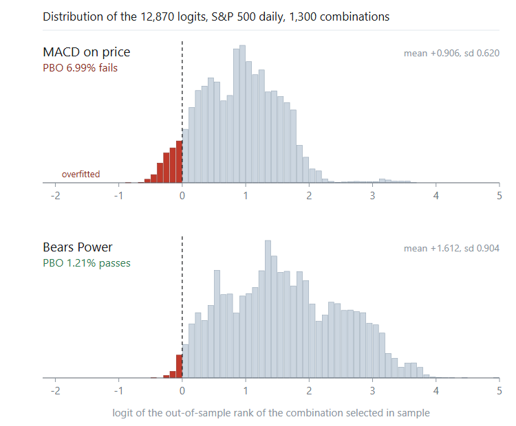
Now put the two out-of-sample numbers side by side.

	MACD on price	Bears Power
PBO	6.99%, fails	1.21%, passes
Out-of-sample return on the best split	20.9%	18.3%

On its own best split, the indicator with the lower PBO produced the worse result, which is not a contradiction but the single most misread point in the literature. The PBO measures the reliability of the selection procedure, not the profitability of what it selects. A low PBO says that the combination chosen in-sample usually stays in the upper half of the same grid out-of-sample, and it says nothing about how much of that combination’s in-sample return survives or whether the combination beats holding the index.

Holding the index returned 44.1% and 42.4% over the out-of-sample halves of those two best splits, one for each indicator, so both selections came in below half of what doing nothing would have paid, although each still beat most of its own grid there. Across all 12,870 splits, the Bears Power selection finished above the median of the grid on 98.8% of them, which is its PBO read the other way, but it beat holding the index over the same half on only 58.8%, and for the MACD on price those two figures are 93.0% and 1.4%.

The low PBO of Bears Power comes with a reservation, because three of its five most selected combinations use a period of 2 with only 20 to 30 position changes over 3,610 bars, and together they account for 40.8% of the splits. A strategy that barely departs from buy and hold will mechanically obtain a flattering number, since there is very little selection happening at all. These low-activity columns also tie for the best in-sample value on more than half of the splits, and the engine then keeps the first of them in column order, which is the one with the shortest period, so this tie rule adds to the weight of period 2 in that list. Choosing among the tied columns at random instead gives an expected PBO of 1.66%, and always keeping the last one gives 4.77%, so Bears Power passes under each rule but with less room than 1.21% suggests, while the MACD on price stays between 6.92% and 7.15% and fails under each.

The degradation plot, and why it needs a control

The obvious next question is whether a better in-sample half predicts a worse out-of-sample half. Plot one against the other, one point per split, and read the slope. Bailey and his co-authors call this performance degradation, and it is a standard part of the framework.

The correlations came out at -0.273 for the MACD on price and -0.792 for Bears Power. Both negative, the second strongly so. Read at face value, that says the better the backtest looked, the worse the result, and for Bears Power it says it emphatically.

That plot has a problem, and it shows in the shape of the cloud, because the points do not scatter at random but fall on clean curves.

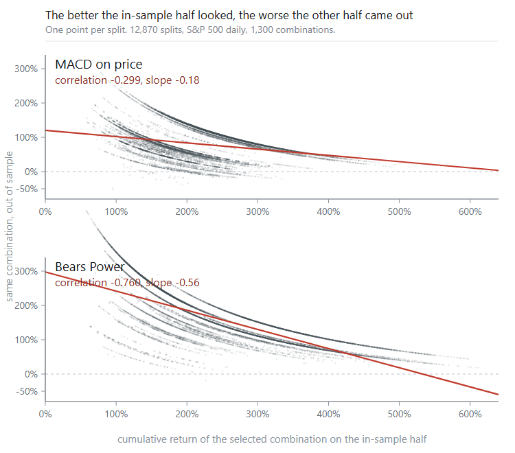
The reason is an identity. The two halves partition the same period, and a cumulative log return is additive, so for any given combination:

IS + OOS = total over the whole sample, which is a constant for that combination

Within one combination, the correlation between the two halves is therefore exactly -1, by arithmetic. Each curve in the figure is one combination, tracing out the ways a fixed total can be divided, and any scatter of this kind inherits that no matter what selection rule produced it.

So how much of -0.792 is a measurement, and how much is bookkeeping?

The way to find out is a control. Walk exactly the same 12,870 splits, but instead of taking the best in-sample combination, take one at random. Whatever slope that produces is the part that does not come from the choice made on each split. The function below is Enumerate with the search for the best column replaced by a draw, and it reuses the same pre-aggregated sums, so it costs one extra pass over data that is already in memory.

//+------------------------------------------------------------------+
//| Control experiment: walk exactly the same splits, but instead of |
//| taking the best trial in sample, take one at random from a pool. |
//|                                                                  |
//| pool[]  column indices the control is allowed to draw from       |
//| seed    fixed so the control is reproducible                     |
//+------------------------------------------------------------------+
bool CCSCVEngine::RunControl(const int &pool[], const int seed,
                             double &outIS[], double &outOOS[])
  {
   if(!m_ready)
      return(false);

   const int poolSize = ArraySize(pool);
   if(poolSize < 1)
      return(false);

   const int  S    = m_partitions;
   const int  N    = m_cols;
   const int  half = S / 2;
   const uint end  = (uint)1 << S;

   double is[];
   if(ArrayResize(is, N) != N)
      return(false);
   if(ArrayResize(outIS,  m_combinations) != m_combinations) return(false);
   if(ArrayResize(outOOS, m_combinations) != m_combinations) return(false);

   MathSrand(seed);
   int c = 0;

   for(uint mask = 0; mask < end && c < m_combinations; mask++)
     {
      if(PopCount(mask) != half)
         continue;

      ArrayInitialize(is, 0.0);
      for(int s = 0; s < S; s++)
        {
         if((mask & ((uint)1 << s)) == 0)
            continue;
         const int base = s * N;
         for(int n = 0; n < N; n++)
            is[n] += m_part[base + n];
        }

      const int pick = pool[MathRand() % poolSize];
      outIS[c]  = is[pick];
      outOOS[c] = m_total[pick] - is[pick];
      c++;
     }

   return(c == m_combinations);
  }

The first control was a surprise.

control, random over all 1,300 combinations : +0.811

Strongly positive, so the identity does not dominate after all. Across the full grid, combinations differ enormously in their total return over fourteen years, and a combination with a high total is good on both halves. That variation between combinations swamps the trade-off within them.

The negative sign only appears once you restrict the draw to the combinations that selection actually visits. Those have similar totals, so the variation between combinations becomes small next to the identity, which forces the two halves apart. That pool is exactly what GetSelected gives you.

//--- build the control pool from the combinations selection actually visits
int sel[];
engine.GetSelected(sel);

bool seen[];
ArrayResize(seen, N);
ArrayInitialize(seen, false);
for(int i = 0; i < ArraySize(sel); i++)
   seen[sel[i]] = true;

int pool[];
ArrayResize(pool, 0);
for(int n = 0; n < N; n++)
  {
   if(!seen[n])
      continue;
   const int k = ArraySize(pool);
   ArrayResize(pool, k + 1);
   pool[k] = n;
  }

double cIS[], cOOS[];
engine.RunControl(pool, 20260816, cIS, cOOS);
PrintFormat("control over the %d ever selected: %.3f",
            ArraySize(pool), Correlation(cIS, cOOS));

Correlation there is an ordinary Pearson correlation over two arrays, which lives in the script rather than in the engine, since the engine returns raw distributions and leaves the statistics to the caller.

With that in hand, the comparison can be made.

	Real selection	Control, same pool	Difference
MACD on price	-0.273	-0.268	0.005
Bears Power	-0.792	-0.545	0.247

• For the MACD on price, selecting the best in-sample combination gives almost the same answer as picking at random from the same pool, which, read at face value, would mean that nearly the whole negative slope is arithmetic plus the narrowing of the pool.
• For Bears Power, the real selection sits a quarter of a correlation point below its control, which, read at face value, would mean that choosing the best in-sample combination damages the out-of-sample result beyond what the identity forces.

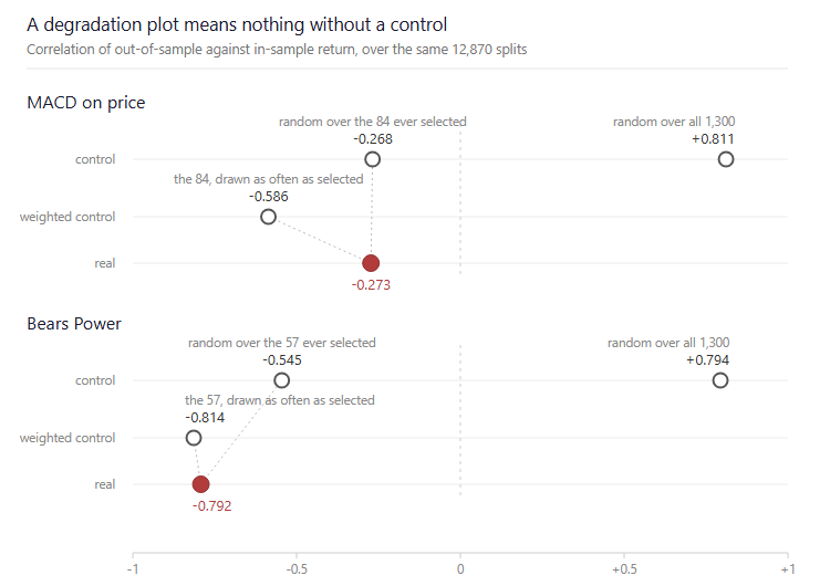
Neither reading survives a second control, because a uniform draw gives every visited combination the same weight while selection keeps returning to a few of them. With sel itself passed to RunControl as the pool, each combination is drawn about as often as selection chose it, on the same 12,870 splits, and that control gives -0.814 for Bears Power, slightly below the real selection, since five combinations with similar totals take 63% of its splits and on those the identity dominates. The same control gives -0.586 for the MACD on price, so changing nothing but the weighting of the pool moves the control by about 0.3 on both indicators, and a gap against a single control is not evidence of a selection effect in either direction.

A degradation plot without a control cannot be interpreted, and that holds well beyond these two indicators. A correlation of -0.792 looks damning until you learn that a random draw from the same pool already gives -0.545. The control costs one extra pass over data that is already in memory, and neither the original paper nor the work that reproduces it publishes one.

How much history a sweep really needs

The same authors give a second result. For a sweep of N independent trials, the history needed before the best trial stops being a mirage has a simple upper bound:

MinBTL < 2 * ln(N) / E[max Sharpe]^2

The Sharpe ratio in that formula is the return of a strategy divided by how much that return varies from one period to the next, and 1 is roughly the level a strategy has to reach to be worth trading. E[max Sharpe] is the annualized Sharpe ratio you want the best of your N trials to show in the backtest, and MinBTL is the number of years below which N trials with no skill at all would be expected to show that much by luck alone. With 1,300 combinations counted as independent trials and a target Sharpe of 1, the bound comes out at about 14.3 years, and the broker provides fourteen. If fourteen years of daily data on the most documented index in the world is marginal on that count, then two years of hourly data on an exotic pair, optimized over 10,000 passes, does not have enough data behind it to mean anything, because the formula counts years and not bars, and two years at a Sharpe of 1 cover only a handful of independent trials.

Applied with N equal to the grid size, though, the formula is too strict, because its derivation assumes the N trials are independent. In a parameter sweep, they are far from independent, since a period of 12 and a period of 13 produce almost the same series of returns. The 1,300 combinations are not 1,300 independent experiments but a much smaller number of distinct ideas sampled at slightly different settings.

The same objection is commonly raised against the standard statistical fix for testing many things at once, the Bonferroni correction, which divides the significance level you demand by the number of tests you ran. On the grid used here, it would demand 5% divided by 1,300, so about 0.004%, which over fourteen years of daily data means an annualized Sharpe ratio of about 1.05, more than any of the 1,300 combinations reaches on either indicator. It gets there by counting a period of 12 and a period of 13 as two separate experiments. The identical objection applies to the minimum backtest length, and it is made far less often.

Counting how many ideas a grid really contains

The honest version replaces N with an effective number of independent trials, meaning how many genuinely different strategies the grid contains rather than how many settings were tried. If every column of the matrix produced the same series of returns, the grid would be one idea tested 1,300 times. If no two columns resembled each other, it really would be 1,300 experiments. The truth sits between the two, and the returns matrix is already built, so measuring where costs nothing extra.

The usual measure is the participation ratio, and it has a form that needs no heavy linear algebra. Write c(i,j) for the correlation between column i and column j, then:

N_eff = N^2 / sum over all i and j of c(i,j)^2

Check that against the two extremes. If the columns are all independent, every correlation off the diagonal is zero and the double sum is just the N ones on the diagonal, so N_eff = N^2 / N = N. If the columns are all identical, every correlation is 1 and the double sum is N^2, so N_eff = 1. Between those two, the more the columns move together, the smaller the answer. Because the correlation is squared, a rule and its mirror image, long whenever the other is short, also count as one idea, although picking the better of the two on the in-sample data gives luck two chances rather than one. The grids here contain pairs close to that, since the columns at their lowest thresholds are almost always long and those at their highest almost always short, so on them the count comes out on the low side.

Here is the full function. It standardizes each column once, then accumulates the squared correlations without ever forming the N by N matrix, which matters at N = 1,300 where that matrix would hold 1.7 million entries.

//+------------------------------------------------------------------+
//| Effective number of independent trials in a T x N returns matrix.|
//|                                                                  |
//| Participation ratio on the correlation matrix, computed without  |
//| an eigendecomposition. For a symmetric matrix the sum of squared |
//| eigenvalues equals the sum of squared entries, and the diagonal  |
//| of a correlation matrix is all ones, so the eigenvalues sum to N:|
//|                                                                  |
//|   N_eff = (sum of eigenvalues)^2 / sum of squared eigenvalues    |
//|         = N^2 / sum_ij c(i,j)^2                                  |
//|                                                                  |
//| data[]  T x N, row-major, the same matrix given to the engine    |
//|                                                                  |
//| Returns N_eff over the columns that vary, or -1.0 on error.      |
//+------------------------------------------------------------------+
double EffectiveTrials(const double &data[], const int rows, const int cols)
  {
   if(rows < 2 || cols < 1 || ArraySize(data) != rows * cols)
      return(-1.0);

   //--- standardise every column: zero mean, unit standard deviation
   double z[];
   if(ArrayResize(z, rows * cols) != rows * cols)
      return(-1.0);

   int live = 0;                               // columns that vary
   for(int n = 0; n < cols; n++)
     {
      double sum = 0.0, sumSq = 0.0;
      for(int t = 0; t < rows; t++)
        {
         const double v = data[t * cols + n];
         sum   += v;
         sumSq += v * v;
        }

      const double mean = sum / rows;
      const double var  = sumSq / rows - mean * mean;
      const double sd   = (var > 0.0) ? MathSqrt(var) : 0.0;
      if(sd > 0.0)
         live++;

      // A column with no variation carries no information. It is left
      // at zero and not counted, so it adds nothing below, neither a
      // correlation nor a one on the diagonal.
      for(int t = 0; t < rows; t++)
         z[t * cols + n] = (sd > 0.0) ? (data[t * cols + n] - mean) / sd : 0.0;
     }

   if(live < 1)
      return(-1.0);

   //--- sum of squared correlations, using the symmetry of the matrix
   double acc = (double)live;                  // one per column that varies
   for(int i = 0; i < cols; i++)
     {
      for(int j = i + 1; j < cols; j++)
        {
         double c = 0.0;
         for(int t = 0; t < rows; t++)
            c += z[t * cols + i] * z[t * cols + j];
         c /= rows;

         acc += 2.0 * c * c;                   // c(i,j) and c(j,i)
        }
     }

   return((double)live * (double)live / acc);
  }

One warning on the cost, since it is nothing like the engine. On the 3,610 by 1,300 matrix used here, the inner loop runs about three billion times, so expect tens of seconds rather than 0.2 seconds.

Feed it the same matrix you gave the engine, put its answer back into MinBTL in place of N, and you get the history required for the number of ideas you actually tested rather than for the number of settings you typed. To take a round illustration and not a measurement, a grid of 1,300 settings that resolved to thirty independent ideas would move the requirement from 14.3 years down to 6.8, which turns fourteen years of history from marginal into comfortable.

Running that on the two grids of this article, and checking how the answer moves when the threshold step is made finer or coarser, is the subject of the second part.

Limitations

The procedure does not judge whether your backtest was honest, since it knows nothing about transaction costs, slippage or whether the data was available at the time. A low PBO on a backtest that ignores the spread only tells you that the selection was stable, and the backtest itself can still be wrong. The runs in this article ignore costs, and charging a spread of half an index point on every position change, about the average the broker lists for this CFD, moves the PBO of the MACD on price from 6.99% to 5.70%, and a full point moves it to 4.50%, while Bears Power goes from 1.21% to 0.82% and 0.55%. The costs lower the PBO because they fall hardest on the combinations that trade most, and in the failing splits those are mostly the pick itself for Bears Power and the columns that beat it for the MACD on price. Overnight financing and dividend adjustments are not modelled either, and since a CFD applies them differently to a long and a short position, they could also shift the comparison.

It cannot see structural breaks that are absent from the sample, so if the regime you will trade in has no counterpart in the history you tested, no cross-validation of that history will warn you. It is not an out-of-time test either, because all but one of the 12,870 splits train on at least one block that comes after a block they test, so CSCV complements a walk-forward test or a forward test on later data rather than replacing it.

Hidden trials break it. Run 1,300 combinations, quietly drop the 800 that looked bad, compute the PBO on the remaining 500, and the number will be flattering and meaningless.

Both verdicts also depend on how the grid is built, because every column competes in the out-of-sample ranking. Reading the range from the longest period leaves the shorter periods with many columns that change position fewer than 30 times and stay close to permanently long or permanently short, and the long ones often beat the selected combination out-of-sample. Giving each period its own range removes almost all of them and brings the MACD on price from 6.99% to 3.89% and Bears Power from 1.21% to 1.59%, while keeping the longest period but reading its range at the 0.5th and 99.5th percentiles takes them to 16.36% and 12.20%. The range is also read from the whole history, so the testing halves help to place it, and reading it from the training half alone on every split gives 5.77% and 3.28%.

Everything above was computed on one instrument, one timeframe, one strategy design and two indicators, so it demonstrates a method rather than establishing a fact about markets, or about how well the PBO separates strategies in general, which would need many more grids, instruments and timeframes.

And the warning that matters most comes from the authors themselves, who write that using the PBO as a criterion to select a strategy is a gross misuse of the method, since any anti-overfitting technique used to select an optimal strategy will itself overfit. The 5% rule from the introduction is a verdict on a procedure fixed before the number is seen, while changing the indicator, the grid or the sample period until the number falls under 5% turns the PBO into that selection criterion, and every one of those changes is a hidden trial in the sense above. The two indicators here are compared to show the measure at work, not to pick the one to trade. Measure, then accept or reject, and never optimize against this number. Strathern put the same idea more generally: when a measure becomes a target, it ceases to be a good measure.

Conclusion

The engine takes a returns matrix and gives back a number in 0.2 seconds, so there is no reason not to run it on your own sweeps.

What it tells you is narrower than it first appears. It will not tell you whether a strategy is good, only whether the combination your process picked in-sample usually stayed in the upper half of the grid on the data it had not seen. That is measured within the history you tested, so it holds for tomorrow only as far as tomorrow resembles that history.

On the data and the grid used here, one indicator failed that test and one passed, and even the one that passed beat holding the index over the same half on only 58.8% of the splits. Neither of those is visible from the backtest itself, which is why both numbers have to be computed.

Two of the findings above were not in the plan when this started. The first is that a low PBO says nothing about profitability, which is the most common misreading of the measure. The second is that a performance degradation plot cannot be interpreted without a control, because a large part of its slope is arithmetic. Both came out of running the code rather than reading about it, which is the best argument I know for implementing a method yourself instead of trusting a summary of it.

All source code is published on MQL5 Algo Forge.

References

• Bergerat, J. (2020), On the Relevance of Optimizing Technical Indicators on U.S. Stock Markets, University of Lausanne, 70 pages. Written 1 June 2020, posted on SSRN 30 April 2025. 
• Bailey, Borwein, López de Prado, Zhu (2015), The Probability of Backtest Overfitting, Journal of Computational Finance
• Bailey, Borwein, López de Prado, Zhu (2014), Pseudo-Mathematics and Financial Charlatanism, Notices of the AMS 61(5)
• Harvey, Liu, Zhu (2015), … and the Cross-Section of Expected Returns
• Strathern (1997), Improving Ratings: Audit in the British University System, European Review 5

Programs used in the article

#	Name	Type	Description
1	CSCVEngine.mqh	Class Library	The CSCV engine. Takes a returns matrix and returns the Probability of Backtest Overfitting. Depends on nothing but the standard library
2	MACDp.mqh	Class Library	MACD on price: distance of the close to its own SMA, optionally as a percentage
3	BearsPower.mqh	Class Library	Bears Power: distance of the low to an EMA of the close, optionally as a percentage
4	RunPBO.mq5	Script	Builds the 1,300-column returns matrix on the chart symbol, runs the engine and the control experiments, exports CSVs
5	TestCSCVEngine.mq5	Script	Two known-answer validation cases: pure noise and one planted winner
6	ExportBars.mq5	Script	Exports the bar history of the chart it is dropped on to CSV, used to draw the article figures
7	MQL5.zip	Archive	An archive of the files above for unpacking into the MQL5 directory of the client terminal