Forecasting a Conditional Distribution Using MLP

Introduction

In the highly volatile and uncertain financial markets such as Forex, accurately predicting price movements remains a key challenge for traders and analysts. Traditional regression approaches based on standard loss functions such as mean squared error (MSE) or sum of squared errors (SSE) often underperform. These functions assume homoscedasticity, that is, constancy of the variance of the target variable, which rarely corresponds to the real dynamics of financial time series. To adequately model such data, an approach is required that takes into account heteroscedasticity — the variable variance of price increments that depends on the input features.

The article presents a probabilistic approach to the regression problem using a multilayer perceptron (MLP) to predict the conditional Gaussian distribution of price increments. For this purpose, we implement a custom loss function based on the Gaussian negative log-likelihood (GaussianNLLLoss).

To implement this approach, the MLPRegressor class was created, integrated with the ALGLIB library, which provides the L-BFGS optimization algorithm. The article describes in detail the key methods of the class — forward and backward propagation, integration with L-BFGS, and an indicator demonstrating the application of the model to forecasting price increments on currency pairs along with an uncertainty estimate. Ultimately, our model provides the trader with not just a point forecast, but the full conditional distribution of the target variable.

MSE loss function and its relationship to the constant-variance Gaussian likelihood

First, let's recall what a loss function is and why it plays a key role in machine learning problems. The loss function is a measure that quantifies how much the model's predictions deviate from the actual data. One of the most common loss functions for regression problems is the Mean Squared Error (MSE), which is calculated as:

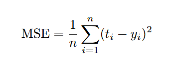
where:

• t — true value of the target variable (target), 
• y — value predicted by the model, 
• n  — number of observations.

The mean squared error (MSE), often used in regression problems, assumes that the target variable follows a normal distribution model with constant variance σ2:

t  ~ N (y, σ2)

Then the likelihood function for a sample of n observations for this model is expressed as the product of the densities of the normal distribution:

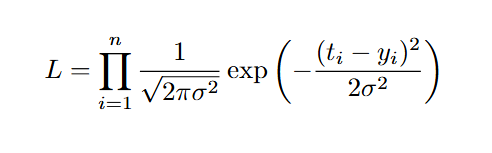
For ease of optimization, the negative log-likelihood is usually minimized:

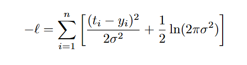
Since the variance σ2 is a constant, the second term in the formula does not depend on the model parameters and does not affect the optimization. Thus, minimizing the likelihood function becomes equivalent to minimizing the MSE. This shows that using MSE as a loss function implicitly assumes that price increments are normally distributed with constant variance independent of the input features.

However, in the context of financial data, such as price increments in Forex currency pairs, this assumption rarely matches reality. In such circumstances, using MSE as a loss function is too simplistic and may lead to insufficiently accurate models that do not take into account changing volatility. To overcome this limitation, we construct a custom loss function based on the Gaussian negative log-likelihood, which models the conditional variance depending on the input features.

Gaussian likelihood with GaussianNLLLoss varying variance

In this case, we assume that the target variable t follows a normal distribution with conditional variance σi2 that depends on the input data xi.

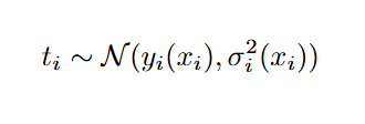
Then the negative logarithm of the likelihood averaging over n observations is expressed as:

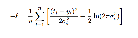
This loss function consists of two terms. The first term is essentially the weighted mean squared error. The weight of each term is inversely proportional to the predicted variance. This means that the higher the predicted uncertainty (σ2), the smaller the influence of the corresponding error on the overall loss function.

The second term prevents the model from trivially inflating σi2 to minimize the first term. It encourages the model to predict a variance that matches the actual uncertainty in the data.

Thus, the GaussianNLLLoss function allows us to simultaneously predict two quantities: the conditional expectation μi and the variance σi2. This is equivalent to modeling a full normal distribution for each data point.

//+------------------------------------------------------------------+
//| GaussianNLLLoss (Negative Log-Likelihood)                        |
//+------------------------------------------------------------------+
double GaussianNLLLoss(const matrix &output, const matrix &target, int sample)
  {
   if(output.Rows() != 2 || output.Cols() != sample || target.Rows() != sample || target.Cols() != 1)
     {
      Print("GaussianNLLLoss: Invalid matrix dimensions");
      return DBL_MAX;
     }

   vector mu = output.Row(0);
   vector sigma2 = output.Row(1); // after softplus

// Limit the dispersion from below by eps value
   for(int i = 0; i < sample; i++)
     {
      sigma2[i] = MathMax(sigma2[i], 1e-6); // max(sigma_i^2, eps)
     }

//  target - mu
   vector diff = target.Col(0) - mu;
//  (t - mu)^2 / (2 * sigma^2)
   vector term1 = diff * diff / (2.0 * sigma2);
//  0.5 * log(2 * PI * sigma^2)
   vector term2 = 0.5 * (MathLog(2.0 * M_PI * sigma2));
// Sum both terms and average
   double sum = (term1 + term2).Sum();
   return sum / sample;
  }

The concept of likelihood

Likelihood is a fundamental concept in statistics, used in both frequentist and Bayesian approaches. It characterizes the probability of observed data considering the given model parameters. In the context of machine learning, likelihood is a measure of how well a model describes the data.

Consider, for example, a data set that is assumed to follow a normal distribution with mean μ and variance σ2. The likelihood function indicates how likely it is that the observed data were generated by a normal distribution with specific values of these parameters. In other words, it helps answer the question: "To what extent do the selected parameters correspond to the observed data?"

To illustrate the maximum likelihood principle, one can run a script that plots the log-likelihood of a sample from a normal N(0,1) distribution against the mean. For a fixed variance σ2=1, the values of μ in the range [−3,3] are tried, and the likelihood is calculated using the MathProbabilityDensityNormal function. The resulting graph shows that the maximum likelihood is achieved at a value of μ≈0, corresponding to the true sample mean. All other values of μ have lower likelihood, indicating that they fit the data less well.

#include <Math\Stat\Normal.mqh>
#include <Graphics\Graphic.mqh>

//+----------------------------------------------------+
//| Log-Likelihood                             |
//+----------------------------------------------------+
double LogLikelihood(const double &t[], double mu, double sigma)
{
   int n = ArraySize(t);
   double result[];
   ArrayResize(result, n);
   // Calculate the logarithm of the probability density
   MathProbabilityDensityNormal(t, mu, sigma, true, result);

   // Sum ln(p(x_i)) to get the log-likelihood
   double ll = 0.0;
   for(int i = 0; i < n; i++)
      ll += result[i]; 
  
   return ll;
} 

//+--------------------------------------------+
//| Plot Log-Likelihood                        |
//+--------------------------------------------+
void PlotLL(const double &mu_values[], const double &ll_values[], int sec)
{
   ChartSetInteger(0, CHART_SHOW, false);
   CGraphic graphic;
   ulong width = ChartGetInteger(0, CHART_WIDTH_IN_PIXELS);
   ulong height = ChartGetInteger(0, CHART_HEIGHT_IN_PIXELS);
   graphic.Create(0, "LL_Graphic", 0, 0, 0, int(width), int(height));
   graphic.CurveAdd(mu_values,ll_values, ColorToARGB(clrBlue, 255), CURVE_LINES, "Log-Likelihood");
   graphic.XAxis().Name("Mu");
   graphic.YAxis().Name("Log-Likelihood");
   graphic.BackgroundMain("Log-Likelihood");
   graphic.XAxis().NameSize(18);
   graphic.YAxis().NameSize(18);
   graphic.BackgroundMainColor(ColorToARGB(clrBlack, 255));
   graphic.BackgroundMainSize(24);
   graphic.CurvePlotAll();
   graphic.Update();
   Sleep(sec * 1000);
   ChartSetInteger(0, CHART_SHOW, true);
   graphic.Destroy();
   ChartRedraw(0);
}

//+------------------------------------------------------------------+
//| Script program start function                                    |
//+------------------------------------------------------------------+
void OnStart()
{
   // Generate a synthetic sample
   MathSrand(55); 
   int n = 100; // Number of observations
   double true_mu = 0.0; // True mean
   double true_sigma = 1.0; // Fixed standard deviation
   double t[]; // Sample
   ArrayResize(t, n);
   MathRandomNormal(true_mu, true_sigma, n, t);

   // Range for mu
   double mu_min = -3.0;
   double mu_max = 3.0;
   double mu_step = 0.1;
   int steps = (int)((mu_max - mu_min) / mu_step) + 1;

   double mu_values[];
   double ll_values[];
   ArrayResize(mu_values, steps);
   ArrayResize(ll_values, steps);

   // Calculate log-likelihood for each mu
   double max_ll = -DBL_MAX;
   double best_mu = 0.0;
   for(int i = 0; i < steps; i++)
   {
      mu_values[i] = mu_min + i * mu_step;
      ll_values[i] = LogLikelihood(t, mu_values[i], true_sigma);
      if(ll_values[i] > max_ll)
      {
         max_ll = ll_values[i];
         best_mu = mu_values[i];
      }
   }

   PlotLL(mu_values, ll_values, 10); 

   // Display results
   Print("True mean: mu = ", true_mu);
   Print("Found mean: mu = ", best_mu);
   Print("Maximum log likelihood value: ", max_ll);
}

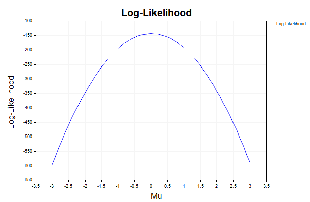
Fig. 1. Plot of the log-likelihood function for the mean N(0,1)

Implementation of the MLP model for a regression problem with the GaussianNLLLoss loss function

To implement the proposed approach to predicting the conditional Gaussian distribution, we will use the multilayer perceptron model (MLPRegressor class). The network architecture is very simple, the model consists of only one hidden layer and has a fixed number of outputs equal to two, where the first output corresponds to the conditional expectation of price increments, and the second to the conditional variance. 

To ensure correct modeling of these parameters, we use fixed activation functions in the output layer: a linear activation for the mean and a Softplus function for the variance, which ensures that the predicted values are positive. The hidden layer activation function can be selected by the user at their own discretion. For a list of all available activation functions, see the "Machine Learning /Activation" MQL5 Help section. 

Two methods play a key role in the operation of the model: forward propagation (FeedForward) and backward propagation (Backprop). The first one computes the predictions μi and σi2 based on the input data, the second one finds the gradients of the GaussianNLLLoss loss function so that the L-BFGS algorithm can update the model parameters.

FeedForward

The FeedForward method implements forward propagation of a signal through a neural network, computing predictions based on input data:

//+------------------------------------------------------------------+
//| Feed forward                                                     |
//+------------------------------------------------------------------+
bool MLPRegressor::FeedForward(const matrix &data)
  {
   ones_ = matrix::Ones(1, data.Rows());
   n1 = weights1.MatMul(data.Transpose()) + bias1.MatMul(ones_);
   n1.Activation(act1, ac_func);
   n2 = weights2.MatMul(act1) + bias2.MatMul(ones_);
   act2.Init(n2.Rows(), n2.Cols());
   act2.Row(n2.Row(0), 0); // First output: linear activation (copy directly)
// Second output: softplus
   vector z = n2.Row(1);
   vector sigma2;
   z.Activation(sigma2, AF_SOFTPLUS);
   act2.Row(sigma2, 1);

   return true;
  }

In the last layer, the network outputs two values: 

• μi — mean obtained directly with linear activation, 
• σi2 — variance that passes through softplus to always remain positive. 

Backprop

The Backprop method implements backpropagation of the error by calculating the gradients of the loss function over all model parameters — weights and biases. These gradients are required to train the model using the L-BFGS algorithm:

//+--------------------------------------------------------+
//| Backprop                                               |
//+--------------------------------------------------------+
bool MLPRegressor::Backprop(const matrix &data, const matrix &target)
  {
   const double eps = 1e-6;     // Parameter for numerical stability of optimization
   vector mu = act2.Row(0);     // mu_i (network output for the mean)
   vector sigma2 = act2.Row(1); // sigma_i^2 (network output for variance)
// Limit sigma2 from below by the value of eps
   for(int i = 0; i < Sample_; i++)
     {
      sigma2[i] = MathMax(sigma2[i], eps); // max(sigma_i^2, eps)
     }
   vector t = target.Col(0);    // t_i (target variable)
   vector diff = t - mu;        // t_i - mu_i

// 1. Gradients of the loss function at the network outputs (mu_i, sigma_i^2)
   matrix DerivLoss_wrt_Output(layer2, Sample_);
   DerivLoss_wrt_Output.Row(-1*diff / sigma2 /Sample_, 0);  // dL/d(mu_i) = -(t_i - mu_i) / sigma^2_i
   vector term = 0.5 / sigma2 - 0.5 * (diff * diff / (sigma2 * sigma2)); // dL/d(sigma_i^2)
   DerivLoss_wrt_Output.Row(term/Sample_, 1); // dL/d(sigma_i^2) = (1/(2*sigma_i^2) - (t_i - mu_i)^2 / (2*sigma_i^2)^2)

// 2. Derivatives of output layer activations
   matrix deriv_act2(layer2, Sample_);
   deriv_act2.Row(vector::Ones(Sample_), 0);
   vector z = n2.Row(1);
   vector sigmoid_z;
   z.Derivative(sigmoid_z, AF_SOFTPLUS);
   deriv_act2.Row(sigmoid_z, 1);

// 3. Output layer error D2
   matrix D2 = deriv_act2 * DerivLoss_wrt_Output; // [layer2, Sample_]

// 4. Derivatives of hidden layer activations
   matrix deriv_act1;
   n1.Derivative(deriv_act1, ac_func); // [layer1, Sample_]

// 5. Hidden layer error D1
   matrix D1 = weights2.Transpose().MatMul(D2); // [layer1, Sample_]
   D1 = D1 * deriv_act1;

// 6. Calculate gradients
   matrix ones = matrix::Ones(Sample_, 1);
   gW1 = D1.MatMul(data);             // Gradients for weights1
   gb1 = D1.MatMul(ones);             // Gradients for bias1
   gW2 = D2.MatMul(act1.Transpose()); // Gradients for weights2
   gb2 = D2.MatMul(ones);             // Gradients for bias2

   return true;
  }

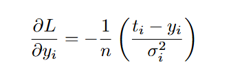
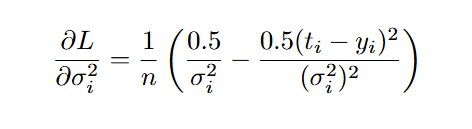
The Backprop method begins by calculating the gradients of the loss function over the network outputs — the mean μi and the variance σi2. Unfortunately, we will not be able to use the built-in LossGradient function from the machine learning section, because it relies on built-in loss functions. Therefore, we should calculate these gradients ourselves using the following formulas.

The gradient of the loss function for the output mean is calculated as:

The gradient of the loss function with respect to the output variance is given by:

The Backprop method is adapted for the GaussianNLLLoss loss function, but its structure is universal. If you want to use a different, non-standard loss function, a key step is to compute the gradients over the network outputs. The remaining steps — activation derivatives and error propagation — follow the standard rules of backpropagation.

Fit method: Training a model with L-BFGS

The Fit method is responsible for training the neural network by combining forward propagation, backpropagation, and parameter optimization using the L-BFGS algorithm.

//+-------------------------------------------------+
//| Fit method using L-BFGS                         |
//+-------------------------------------------------+
bool MLPRegressor::Fit(const matrix &data, const matrix &target)
  {
   Sample_ = (int)data.Rows();
   Features = (int)data.Cols();
   ones_ = matrix::Ones(1, Sample_);

   ArrayResize(target_Plot, Sample_);
   for(int i = 0; i < Sample_; i++)
      target_Plot[i] = target[i, 0];

   if(!CreateNet())
      return false;

// Create an object for optimization
   MLPOptimizationObjective objective(GetPointer(this), data, target);
   MLPReportCallback frep(GetPointer(this)); // Create an object to track the loss function
   CObject obj;

// Prepare parameters
   CRowDouble params;
   objective.PackParameters(params);
   double theta[];
   ArrayResize(theta, params.Size());
   for(int i = 0; i < params.Size(); i++)
      theta[i] = params[i];

// Set up optimization parameters
   double epsg = 0.0001;     // Gradient accuracy
   double epsf = 0.00001;     // Precision by function value
   double epsw = 0.0000;   // Accuracy by parameters
   int maxits = Epochs;       // Maximum number of iterations

// Initialize and start L-BFGS
   CMinLBFGSStateShell state;
   CMinLBFGSReportShell rep;
   CAlglib::MinLBFGSCreate(params.Size(), theta, state);
   CAlglib::MinLBFGSSetCond(state, epsg, epsf, epsw, maxits);
   CAlglib::MinLBFGSSetXRep(state, true); // Enable optimization progress reports
   CAlglib::MinLBFGSOptimize(state, objective, frep, true, obj);
   CAlglib::MinLBFGSResults(state, theta, rep);

//----------TerminationType field contains completion code, which can be:
//  -8    internal integrity control detected  infinite  or  NAN  values  in
//        function/gradient. Abnormal termination signalled.
//   1    relative function improvement is no more than EpsF.
//   2    relative step is no more than EpsX.
//   4    gradient norm is no more than EpsG
//   5    MaxIts steps was taken
//   7    stopping conditions are too stringent,
//        further improvement is impossible,
//        X contains best point found so far.
//   8    terminated    by  user  who  called  minlbfgsrequesttermination().
//        X contains point which was   "current accepted"  when  termination
//        request was submitted.
//--------------------------------------------------------------------------
// Get the final array of parameters
   for(int i = 0; i < (int)params.Size(); i++)
     {
      params.Set(i, theta[i]);
     }
   objective.UnpackParameters(params);

// Final forward pass with optimized parameters
   if(!FeedForward(data))
      return false;

// Save all network outputs in one-dimensional form for later use in the PlotGraphic method
// for visualization. The array contains the parameters of the normal distribution for each observation.
   ArrayResize(NetOutput, Sample_ * layer2);
   for(int i = 0; i < Sample_; i++)
      for(int j = 0; j < layer2; j++)
         NetOutput[i * layer2 + j] = act2.Transpose()[i, j];

   PrintFormat("L-BFGS Optimization completed. Iterations: %d, Termination type: %d, Final loss: %.5f",
               rep.GetIterationsCount(), rep.GetTerminationType(), objective.GetLoss());

   for(int i = 0; i < LossCount; i++)
      PrintFormat("Iteration %d, Loss: %.5f", i, LossPlot[i]);

   return true;
  }

Training is organized as a sequence of the following stages. First, the CreateNet method is called, which initializes the weights (weights1, weights2) and biases (bias1, bias2) matrices with random values, preparing the model for training. An object of class MLPOptimizationObjective is then created, which connects the model to the L-BFGS optimizer, providing the loss function and its gradients.

The model parameters are converted into a one-dimensional 'params' array using the PackParameters method to match the format required by L-BFGS. To monitor convergence, an MLPReportCallback class object is created, which records the values of the loss function in the LossPlot array after each optimization iteration.

Next, the L-BFGS algorithm is configured using the optimization parameters:

• epsg — accuracy by the gradient norm, which determines the stopping criterion by the smallness of the gradients,
• epsf — accuracy by the loss function value,
• epsw — accuracy by parameter changes,
• maxits — maximum number of iterations corresponding to the user-specified number of epochs.

Optimization is started with an initial parameter vector via the MinLBFGSCreate and MinLBFGSOptimize functions. Activating the MinLBFGSSetXRep(state, true) function calls the virtual Rep method of the MLPReportCallback class to save the history of the loss function values. Once the optimization is complete, the final parameters are extracted into the theta array using MinLBFGSResults and unpacked back into weight and bias matrices. After this, a final forward pass is performed through the FeedForward method to obtain the model predictions. These results are stored in the NetOutput array for later analysis or visualization.

Why was L-BFGS chosen?

L-BFGS was chosen for training the MLPRegressor model because it handles user-defined loss functions without issue, unlike the Levenberg-Marquardt algorithm, which is limited to only quadratic functions like MSE.

Stochastic gradient methods such as Adam are the optimal and often the only choice for training neural networks with many hidden layers on large data sets where huge amounts of information need to be processed. However, in the context of quote analysis, where relatively small data sets are used, due to the rapid decay of memory of past events, these methods are significantly inferior in convergence speed to second-order methods such as L-BFGS.

Classes for integration with the L-BFGS optimizer

To connect our class with the optimization method, two auxiliary classes are implemented: MLPOptimizationObjective and MLPReportCallback. We use them to feed loss functions and gradients into the optimizer and to track optimization progress. 

MLPOptimizationObjective class

The MLPOptimizationObjective class connects the MLPRegressor neural network with the L-BFGS optimization algorithm from the ALGLIB library. Inheriting from CNDimensional_Grad, it overrides the virtual function Grad to provide L-BFGS with the GaussianNLLLoss loss function value and its gradients needed for training.

//+------------------------------------------------------------------+
//| Class for the L-BFGS optimizer objective function                |
//+------------------------------------------------------------------+
class MLPOptimizationObjective : public CNDimensional_Grad
  {
private:
   MLPRegressor*     m_mlp;  // Pointer to the neural network object
   matrix            m_data;        // Input data
   matrix            m_target;      // Target values
   double            m_loss;        // Current losses

public:
                     MLPOptimizationObjective(MLPRegressor* mlpLBFGS, const matrix &data, const matrix &target)
      :              m_mlp(mlpLBFGS), m_data(data), m_target(target), m_loss(0.0) {}

   double            GetLoss() { return m_loss; }

   // Method for converting parameters to a one-dimensional array
   void              PackParameters(CRowDouble &params)
     {
      int total_params = (int)(m_mlp.GetNumNeuronsLayer1() * m_data.Cols() +     // weights1
                               m_mlp.GetNumNeuronsLayer1() +                     // bias1
                               m_mlp.GetNumNeuronsLayer2() * m_mlp.GetNumNeuronsLayer1() + // weights2
                               m_mlp.GetNumNeuronsLayer2()) ;                     // bias2
      params.Resize(total_params);

      int idx = 0;
      //  weights1
      for(int i = 0; i < m_mlp.GetNumNeuronsLayer1(); i++)
         for(int j = 0; j < (int)m_data.Cols(); j++)
            params.Set(idx++, m_mlp.weights1[i,j]);

      //  bias1
      for(int i = 0; i < m_mlp.GetNumNeuronsLayer1(); i++)
         params.Set(idx++, m_mlp.bias1[i,0]);

      //  weights2
      for(int i = 0; i < m_mlp.GetNumNeuronsLayer2(); i++)
         for(int j = 0; j < m_mlp.GetNumNeuronsLayer1(); j++)
            params.Set(idx++,m_mlp.weights2[i,j]);

      //  bias2
      for(int i = 0; i < m_mlp.GetNumNeuronsLayer2(); i++)
         params.Set(idx++,m_mlp.bias2[i,0]);
     }

   // Method for unpacking parameters from a one-dimensional array
   void              UnpackParameters(const CRowDouble &params)
     {
      int idx = 0;
      //  weights1
      for(int i = 0; i < m_mlp.GetNumNeuronsLayer1(); i++)
         for(int j = 0; j <(int) m_data.Cols(); j++)
            m_mlp.weights1[i,j] = params[idx++];

      //  bias1
      for(int i = 0; i < m_mlp.GetNumNeuronsLayer1(); i++)
         m_mlp.bias1[i,0] = params[idx++];

      //  weights2
      for(int i = 0; i < m_mlp.GetNumNeuronsLayer2(); i++)
         for(int j = 0; j < m_mlp.GetNumNeuronsLayer1(); j++)
            m_mlp.weights2[i,j] = params[idx++];

      //  bias2
      for(int i = 0; i < m_mlp.GetNumNeuronsLayer2(); i++)
         m_mlp.bias2[i,0] = params[idx++];
     }

   virtual void      Grad(CRowDouble &params, double &func, CRowDouble &grad, CObject &obj) override
     {
      UnpackParameters(params);

      // Feed forward
      if(!m_mlp.FeedForward(m_data))
        {
         func = DBL_MAX;
         for(int i = 0; i < params.Size(); i++)
            grad.Set(i, DBL_MAX);
         return;
        }

      // Calculate the loss function
      func = GaussianNLLLoss(m_mlp.act2, m_target,(int) m_data.Rows());
      m_loss = func;

      // Perform backpropagation to obtain gradients
      if(!m_mlp.Backprop(m_data, m_target))
        {
         func = DBL_MAX;
         for(int i = 0; i < params.Size(); i++)
            grad.Set(i, DBL_MAX);
         return;
        }

      // Form a gradient vector
      int idx = 0;

      for(int i = 0; i < m_mlp.GetNumNeuronsLayer1(); i++)
         for(int j = 0; j <(int) m_data.Cols(); j++)
            grad.Set(idx++, m_mlp.gW1[i,j]);

      for(int i = 0; i < m_mlp.GetNumNeuronsLayer1(); i++)
         grad.Set(idx++, m_mlp.gb1[i,0]);

      for(int i = 0; i < m_mlp.GetNumNeuronsLayer2(); i++)
         for(int j = 0; j < m_mlp.GetNumNeuronsLayer1(); j++)
            grad.Set(idx++, m_mlp.gW2[i,j]);

      for(int i = 0; i < m_mlp.GetNumNeuronsLayer2(); i++)
         grad.Set(idx++, m_mlp.gb2[i,0]);
     }
  };

L-BFGS works with a one-dimensional array of parameters, but our network stores parameters as matrices of weights and bias vectors. Therefore, we vectorize the parameters using the PackParameters function and unpack them back into matrices using the UnpackParameters function. 

The Grad method is the main method called by L-BFGS at each iteration. It is called repeatedly, sometimes tens or hundreds of times per iteration, to estimate the loss function and gradients for different sets of parameters. Therefore, we cannot store the value of the loss function in this method, otherwise we would get a bunch of intermediate values that do not reflect the real learning progress, but only L-BFGS evaluations.

To monitor convergence, a separate MLPReportCallback class is used, which records losses only after the iteration is completed.

MLPReportCallback class

Inheriting from CNDimensional_Rep from the ALGLIB library, our class overrides the virtual function Rep to store the loss function values into the LossPlot array for later model convergence analysis.

//+------------------------------------------------------------------+
//| Class for tracking the network training progress                 |
//+------------------------------------------------------------------+
class MLPReportCallback : public CNDimensional_Rep
  {
private:
   MLPRegressor      *mlp;

public:
                     MLPReportCallback(MLPRegressor *mlp_instance) : mlp(mlp_instance) {}
                    ~MLPReportCallback() {}

   virtual void      Rep(CRowDouble &arg, double func, CObject &obj) override
     {
      if(mlp != NULL)
        {
         ArrayResize(mlp.LossPlot, mlp.LossCount + 1, 10000);
         mlp.LossPlot[mlp.LossCount] = func;
         mlp.LossCount++;
        }
      else
        {
         Print("MLPReportCallback: Invalid pointer to MLPRegressor");
        }

     }
  };

The L-BFGS algorithm calls the Rep method, passing the current model parameters (arg) and the loss function value (func). It is important that the call to Rep occurs only after the completion of a full L-BFGS iteration, and not during intermediate calculations in the Grad method of the MLPOptimizationObjective class. At this stage, it only remains to store the required information in the array, for example the loss value.

Indicator for predicting conditional distribution

To test the MLPRegressor model, we will write an indicator that will predict the conditional expectation of the price increment and the conditional variance.

Indicator inputs:

• InpPeriodWindow — window size for calculating price increments,
• InpSamples — number of training examples,
• InpShift — number of bars to test,
• InpLayer1 — number of neurons in the hidden layer of the network,
• InpEpochs — maximum number of epochs for training the model.

The training and test datasets are generated using the CollectData and CollectTestData functions. Historical closing prices are used for training. The features are a matrix of size nsamples×(window−1), where each row contains price increments for window−1 previous bars. The target variable is a vector of size nsamples×1 containing price increments (close_i − close_i+1).

The data is normalized using the mean (train_data_mean) and standard deviation (train_data_std) calculated on the training set. Normalization stabilizes training by improving model convergence by bringing the input features and the target variable to the same scale. The CollectTestData function generates a test set for the last InpShift bars, applying the same normalization parameters.

In the OnInit function, an instance of the MLPRegressor class is created with the specified hidden layer activation function. After training, the time spent on training and the total number of model parameters are displayed.

In the OnCalculate function, the forecast is performed using the Predict method, and calculations are performed only when a new bar appears.

Fig. 2. EURUSD mean forecast and 95% confidence intervals

Conclusion

In this article, we used a multilayer perceptron model that predicts the parameters of a conditional Gaussian distribution. For this purpose, we applied a custom loss function based on the Gaussian negative log-likelihood. This loss function allows us to effectively model heteroscedasticity of price increments, which is a key advantage over traditional neural network training approaches based on the mean squared error (MSE), which implicitly assumes that the variance of the target variable is constant. 

We described in detail the architecture of the MLPRegressor class, including the forward and backward propagation methods, as well as the integration with the L-BFGS optimization algorithm from the ALGLIB library via the MLPOptimizationObjective and MLPReportCallback classes. 

The indicator, built on the MLPRegressor class, demonstrates the practical applicability of the model, allowing traders to obtain confidence intervals in addition to the average forecast. This allows for more informed decisions by taking into account not only expected price movements but also their uncertainty, which is especially valuable in volatile markets.

It is important to emphasize that training neural networks should not be limited to standard loss functions such as MSE. Experiments with different probability models and likelihood functions open up new possibilities for data analysis. Researchers and practitioners can adapt machine learning models to the unique characteristics of financial markets, leading to improved forecast accuracy and a deeper understanding of market dynamics.