Forecasting in Trading Using Grey Models

Introduction

Modern financial markets are highly volatile and dynamic, so accurate and timely forecasting plays a crucial role in making trading decisions. Every trader strives to develop and apply forecasting methods that allow them to anticipate future price movements and maximize profits.

Technical analysis offers a wide variety of forecasting methods. But many forecasting methods have their limitations. For example, a statistical approach to forecasting requires a large amount of historical data. Other approaches work well only on stationary time series, etc.

In this context, interest in forecasting methods that can handle limited and incomplete information is growing. One such approach is Grey models (GM), which can be very useful in situations where data is limited, unreliable, or noisy. Such situations are quite common in financial markets. In this article, we will review the basics of GM and how they can be applied to financial time series forecasting.

Classic GM(1,1) model

Grey models can be used to solve a wide variety of problems. With the help of GM we can analyze a time series, smooth it or identify the main trends in price movement. But this model can also be used for forecasting. The main advantage of using GM is that this model does not impose any restrictions on the stationarity of the time series. For example, SMA will show all its best qualities if the time series is stationary and its values are normally distributed. If the time series is non-stationary (in other words, there is a trend), then SMA will be hopelessly lagging. For GM, these requirements are not important and it can cope with any time series. Or at least it should. The requirements for GM are simple and easy to fulfill:

• the length of the time series should be at least 4;
• the values of the time series should be strictly positive and occur at equal time intervals, without gaps.

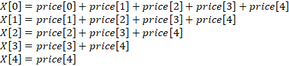
The construction of any GM begins with the application of Accumulated Generating Operation (AGO). The essence of this operation is very simple - you need to sum the current value of the time series with all the previous ones. In the future, I will call such a time series a Grey series (GS). Let's take 5 prices as an example. Then the AGO operation applied to them will look like this:

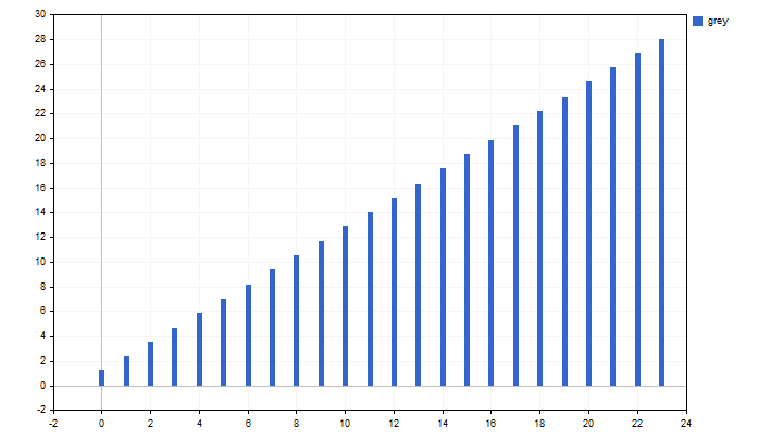
This operation serves two main purposes. First, we reduce the impact of noise. Second, the new time series becomes more predictable – it strictly increases and may look, for example, like this:

Once we have obtained the values of the new time series, we can begin constructing GM(1,1). In this notation, the first number indicates the order of the differential equation, and the second indicates the number of GS being processed. The GM(1,1) model is described by a linear differential equation.

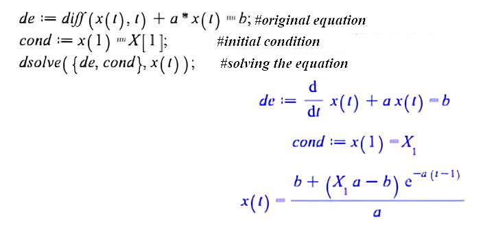
To solve this equation, we need some system of symbolic mathematics. I use Maple. First, we write down the initial equation, then we specify the initial condition and obtain the solution. In Maple, all these operations will look like this:

de:=diff(x(t),t)+a*x(t)=b; #original equation
cond:=x(1)=X[1];           #initial condition
dsolve({de,cond},x(t));    #solving the equation

Thus, we obtained the dependence of the change in GS on time. Please note that the t index represents time and increases from the past to the future, starting from 1. From this equation, we can obtain the same relationship for price change:

In Maple, the solution to this equation would look like this:

eq:=price[t]=(b+(a*X[1]-b)*exp(-a*t))/a-(b+(a*X[1]-b)*exp(-a*(t-1)))/a;#difference between 2 consecutive GS values
simplify(eq);#simplify the result

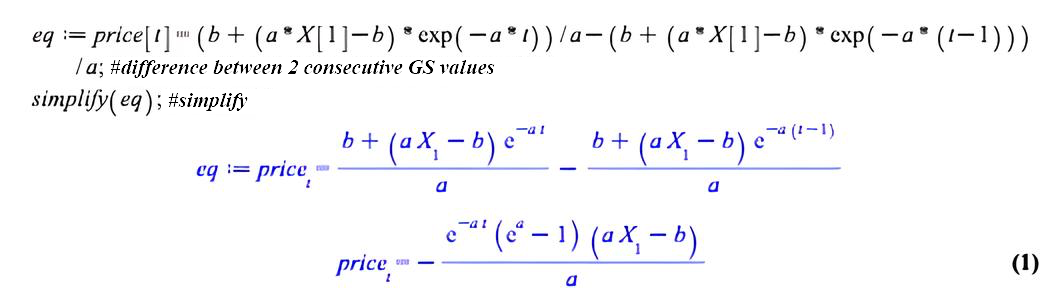
Let's simplify the result a little manually, and the formula will take its final form.

From this formula, it becomes clear that knowing the a and b parameters, we can estimate the price values. In other words, smooth the original time series. In order to estimate these parameters, we need to take the differential equation and discretize it. To do this, we will use the following transition:

After this transition, we get a discrete version.

The coefficients of such an equation can be easily estimated using the least squares method (OLS). This is where the fun begins. We can obtain a smoothed estimate of the GS values. This kind of smoothing is of purely academic interest and is of no practical use.

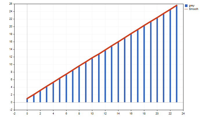
Or we can immediately smooth out the original time series.

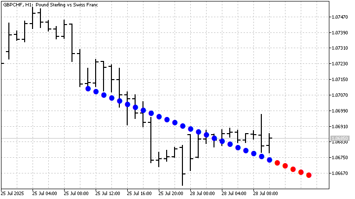
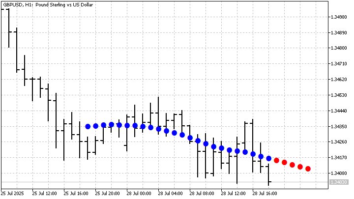
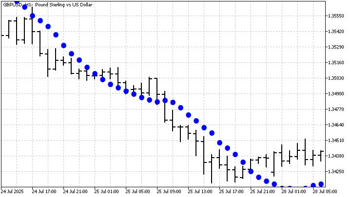
Now we are ready to take the next step. As you might remember, the formula for calculating price values does not impose any restrictions on the increase in time. In other words, we can continue to construct a new time series for as long as we want. In this case, we will get a price movement forecast. Of course, this forecast is based on the assumption that the characteristics of the original time series will remain unchanged. I will make a forecast for 5 steps ahead.

As you can see, this model copes well with linear trends. But because of this, it may miss other important price movements. Let's try to apply more complex GM models and see how they behave.

GM(1,1) modifications

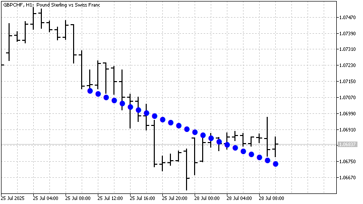
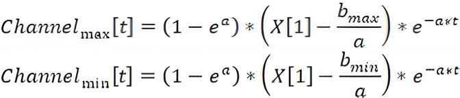
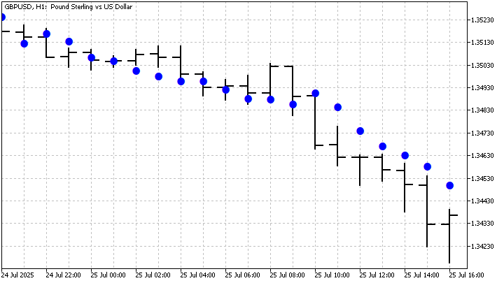
The simplest extension of the classic GM(1,1) is called Rolling GM (RGM). The essence of this extension is very simple. We need to take the values of several GMs with different periods and find their average. With this approach, we can get a smoother estimate of price values. The forecast will also be smoother. Let's make an RGM assembled from several GM(1,1) with periods 4 - 24. This is what it looks like on the chart:

The RGM model can also be modified. The main idea of this modification is to give each GM its own weight. These weights can be either fixed or dependent on the forecast error. The first case is quite trivial. We can assign weights based on arbitrary considerations. We then obtain a weighted sum of the models.

If the weights depend on the forecast error, then you get an adaptive version of RGM. In this case, the weight of each GM can be determined as follows. First, we calculate the forecast error for each GM separately:

The GM weighting factor will depend on this error - the larger the error, the lower the weight:

In this way, RGM will only favor those trends that most closely match the price movement. Accordingly, the quality of the forecast may also improve.

Another complication comes down to the pre-processing of the original time series. For example, instead of prices we can use SMA values. Then GM(1,1) will give smoother results. In practice, this approach can be used to determine trend boundaries.

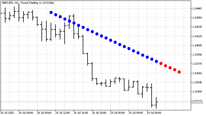
But the channel can be built differently. First, we need to calculate the GM(1,1) parameters. More precisely, now we only need the a growth parameter. Now for each real price value we will calculate its b parameter.

Of all possible options, we are interested in the maximum and minimum values of this parameter. With their help, we can obtain the upper and lower boundaries of the trend channel.

This is what such a channel looks like on a chart:

There are a large number of different modifications of Grey models. Some of these modifications are only applicable to specific time series. Others, like GM(1,1), are universal. All these modifications have one goal - increasing the accuracy of forecasts and identifying the features of time series.

GM discrete models

The solution of differential equations certainly looks beautiful, but even a slight complication of the models leads to very complex solutions. Moreover, the estimation of the model parameters may be numerically unstable. A single error, even deep in the decimal places, may render the chart useless.

Discrete GM variants are free from these drawbacks. Let's try to construct such a variant for GM(1,1). Such a model can be expressed by the following linear recurrence equation:

In other words, we construct a linear dependence of the current value of GS on the previous one. Estimating the parameters of this equation is not difficult. Now we need to find the equation parameters.

re:=x(n+1)=a*x(n)+b;              #original equation

cond:=x(1)=X[1];                  #initial condition
simplify(rsolve({re,cond},x(t))); #solving the equation

As a result, we obtain an equation with explicitly specified GS values.

From this equation, we can obtain a price estimate.

This is what an indicator based on this model looks like:

The experiment was successful. Now let's try to build the GM(0,2) model. From the notation, it is clear that in this model derivatives are not used, and the number of factors taken into account increases. By the way, this model can only exist in a discrete form.

This model uses two GS. Let's assume that the period of the model is N. We build the first GS as usual, starting from the price with index N-1. To construct the second one (I will denote it as Y), we use prices shifted back by 1 count, starting with the price with the index of N. The equation for this model looks like this:

Of course, we can construct a recurrence equation and find its solution. But this model becomes especially simple if we limit ourselves to a 1-step-ahead forecast. So, first we will estimate the model parameters using OLS. We cannot continue the X series - the new price is not yet known. But for series Y the next price is already known, and we can get its new value.

Having obtained a new value for the Y series, we can also estimate the future value of the X series.

After this, making a price forecast will not be difficult. This is what the indicator built on this model looks like:

The GM(0,2) model is similar to linear regression. Increasing the number of GS taken into account can make the model more flexible and improve the forecast quality. This improvement will be especially noticeable with a short indicator period.

We are now ready to move on to constructing the discrete GM(1,2) model. It combines the approaches of the two previous models and can be described by the formula:

In other words, we construct the same linear regression for two GS. We can estimate the future price value using the parameters found for this regression. This is what an indicator based on this model looks like:

The discrete approach makes it quite easy to construct higher order models. As an example, I will take the GM(2,1) model. Solving it in the traditional way, finding the values of its parameters, is not everybody's cup of tea. But let's convert this model into discrete form, then its equation will look like this:

Calculating the parameters of this model will not be difficult. For simplicity, we will also limit ourselves to a forecast one count ahead. On the chart, the indicator looks like this:

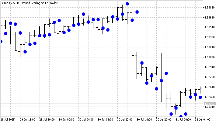
This indicator cannot be called smoothing. But it reacts quite quickly to changes in the market situation. This makes it worth paying attention to. If you want a smoother option, consider using RGM.

To summarize, I can say that discrete models are simpler in their calculations. This is their undoubted advantage. But this simplicity imposes limitations on the forecast horizon. Most often, discrete models only work well one step ahead. Attempts to increase the forecast horizon lead to unnecessary complications and are unlikely to be useful in practice.

Conclusion

Grey models are a promising tool for modeling and describing financial time series. GM can be used for smoothing, trend detection and forecasting of future price values, as well as for constructing trend channels.

The undoubted advantage of GM is the possibility of modifying them to suit almost any external conditions. A serious drawback is the mathematical complexity of some approaches. In any case, GMs require further study and identification of the most suitable options for the trader.

The following programs are attached to the article:

Name	Type	Description
sGM	script	The script demonstrates the construction of GS and smoothing using the GM(1,1) model. If ScreenShot is enabled, the image is saved in the Files folder.
GM11	indicator	The indicator demonstrates the operation of the classic version of GM(1,1) iPeriod - indicator period; Forecast - forecast horizon Shift - indicator shift
RGM11	indicator	The indicator shows the average of several GM(1,1) variants
GM11sma	indicator	Instead of prices, SMA values are used as inputs.
GM11Ch	indicator	The indicator builds a trend channel based on GM(1,1)
DGM11	indicator	Discrete version of GM(1,1)
DGM02	indicator	Analogue of bivariate linear regression
DGM12	indicator	Discrete GM(1,1) model with two input factors
DGM21	indicator	Discrete analogue of the second order model