

Graph Theory: Study of Graphs Generated by Some Random Process
 118
118
 0
0

Table of contents
- Introduction
- System Overview
- Getting Started
- Constants and Inputs
- The State Graph Class
- The K-Step Random Walk
- Binarizing the Network
- Measuring Clustering
- The Erdos–Renyi Null Model
- The Trade-Outcome Graph
- Encoding a Bar into a Vertex
- Building the Graph from History
- Reading the Live Bar
- Position Sizing and Execution
- Managing the Position as a Random Walk
- Closing the Walk
- The Main Loop
- The Dashboard
- Exit Signal
- Backtest
- Conclusion
Introduction
Most trading systems we build carry a hidden assumption. They assume the market has one fixed structure, and that our job is to find it. A moving average crossover assumes trends behave the same way every month. A support and resistance rule assumes a level means the same thing in January and in September. Even the graph algorithms we have already covered in this series, such as Dijkstra, breadth-first search, and A*, work on a graph whose edges are known and stable before the search begins. The trader then spends months tuning parameters, because the fixed map keeps drifting away from the territory. The strategy works for a while, then quietly stops working, and nobody can say exactly when the change happened.
Adaptive models come in many forms, and random graph theory is one of them. It offers a different starting point. Instead of assuming the graph is given, we assume the graph is generated by a random process that we can only observe. Vertices are still market objects, but edges appear and disappear with probabilities that we estimate from data. The network is allowed to rewire itself as the market changes. This is a closer fit to non-stationary markets than a frozen map, although whether it produces a trading edge is something we must test rather than assume. It also gives us something a fixed graph cannot give us, which is a way to ask whether one measurable property of the structure we believe we see differs from chance. If we can generate purely random graphs with the same size and the same expected edge density as our market graph, we can compare them. When our market network looks no different from a coin-flip network on that measure, the structure offers no support for the forecast, and a cautious response is to stay flat.
In this article we build an Expert Advisor around this idea. We discretize the market into a small set of states, let bar-to-bar movement generate edges, and run a random walk on the resulting network to forecast direction. We then subject that network to an Erdos–Renyi null model and can optionally allow trades only when the structure passes the test. Finally, we treat each open position as its own small random walk over R-multiple milestones, and we let the learned survival probabilities decide when to take money off the table. Everything is estimated from the instrument in front of us, and the features are normalized so the same code runs on any symbol. The thresholds, periods, and exit levels are still fixed inputs, however, and they must be validated for each instrument.
System Overview
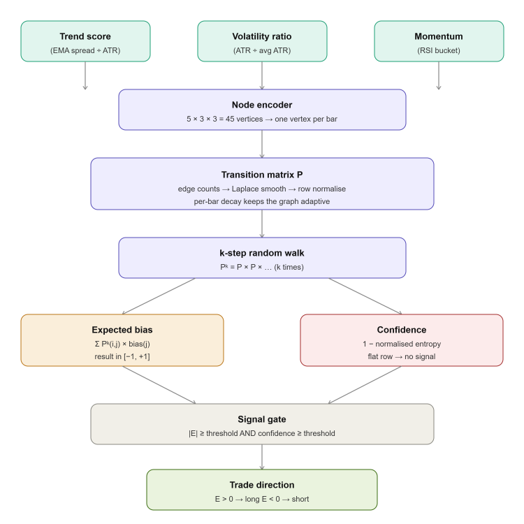
The Expert Advisor maintains two graphs that are learned at the same time. The first is the state-transition network. We describe every closed bar with three dimensionless quantities. The first is the distance between a fast and a slow EMA, divided by ATR, which tells us how strong the trend is in units of current volatility. The second is ATR divided by its own long-run average, which tells us whether volatility is compressed or expanded. The third is RSI, which tells us where momentum sits. Each quantity is placed into a bucket. Five trend buckets, three volatility buckets, and three momentum buckets give us forty-five vertices. When the momentum axis is switched off, the network collapses to fifteen vertices. Every bar the market lands on one vertex, and the jump from the previous vertex to the current one increments one edge.
After enough observations, the edge counts become a transition matrix. Because we apply Laplace smoothing, the matrix is always well defined even when data is thin. Because we decay old counts on every bar, the network forgets slowly and keeps adapting. Raising the matrix to the power of k gives us the k-step walk, which answers a very direct question. Given where the market stands today, where is the process likely to be k bars from now? We attach a directional bias to each vertex (−1 for strong downtrend, +1 for strong uptrend). We then compute the expected bias from the k-step row. That single number, bounded between minus one and plus one, is our signal. We also measure the entropy of the same row. A flat row means the walk has already mixed, the forecast has no information left, and we ignore it.
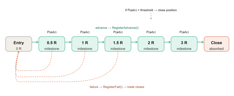
The second graph is the trade-outcome network. Its vertices are R-multiple milestones at 0.5R, 1R, 1.5R, 2R, and 3R, plus an absorbing state that represents the trade ending. Each position is a random walk through these nodes. Every time a trade reaches a milestone, we record an advance on the previous node. Every time a trade dies, we record a failure on the node it died on. The smoothed ratio gives us the probability of surviving one more hop. When that probability drops below a threshold, we treat the next hop as too unlikely to wait for, and we close the position. This is a rule of thumb based on the transition probability alone. A full expected-value test would also weigh the size of the remaining move, the depth of a possible rollback, and trading costs. Even so, it turns exit management into a measured decision rather than a guess.
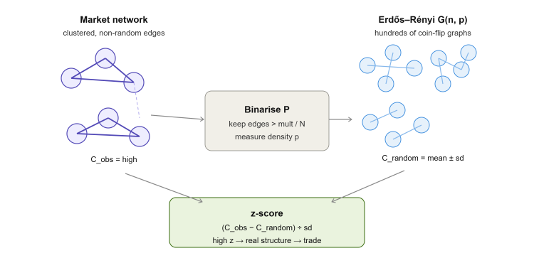
Sitting between the two graphs is the randomness test. We binarize the transition matrix by keeping only edges that are materially stronger than the uniform baseline of one over N. We measure the clustering coefficient of the resulting network. We then generate hundreds of Erdos–Renyi graphs with the same vertex count and the same expected edge density, and we measure their clustering as well. The gap between the two, expressed as a z-score, tells us how far our market network sits from pure randomness on this one metric. A high z-score means the binarized network is more clustered than a random graph of similar density, which is consistent with persistent regimes. A z-score near zero means this metric cannot separate the network from randomness. Neither result proves or disproves a trading edge, so we treat the z-score as an optional filter rather than a forecast.
Getting Started
Constants and Inputs
//+------------------------------------------------------------------+
//|                                         Erdos–Renyi Theory.mq5   |
//|                                  Copyright 2025, MetaQuotes Ltd. |
//|                     https://www.mql5.com/en/users/johnhlomohang/ |
//+------------------------------------------------------------------+
#property copyright "Copyright 2025, MetaQuotes Ltd."
#property link      "https://www.mql5.com/en/users/johnhlomohang/"
#property version   "1.00"
#property description "Random Graph Theory EA: state-transition network + Erdos-Renyi randomness test + trade-outcome graph"

#include <Trade\Trade.mqh>
#include <Trade\PositionInfo.mqh>

//+------------------------------------------------------------------+
//| Constants                                                        |
//+------------------------------------------------------------------+
#define MAX_NODES     45     // 5 trend buckets * 3 volatility buckets * 3 momentum buckets
#define R_LEVELS       5     // number of R milestones in the trade-outcome graph

//+------------------------------------------------------------------+
//| Inputs                                                           |
//+------------------------------------------------------------------+
input group "=== Node Definition (state discretisation) ==="
input int      InpFastEMA            = 21;      // Fast EMA period
input int      InpSlowEMA            = 89;      // Slow EMA period
input int      InpATRPeriod          = 14;      // ATR period
input int      InpRSIPeriod          = 14;      // RSI period
input int      InpVolLookback        = 100;     // Lookback for average ATR (volatility ratio)
input bool     InpUseMomentumAxis    = true;    // Add RSI axis to the node encoding (15 -> 45 nodes)
input double   InpTrendWeak          = 0.25;    // |EMA spread| / ATR : range vs weak trend
input double   InpTrendStrong        = 1.00;    // |EMA spread| / ATR : weak vs strong trend
input double   InpVolLow             = 0.85;    // ATR ratio : low volatility below this
input double   InpVolHigh            = 1.25;    // ATR ratio : high volatility above this
input double   InpRSIBand            = 6.0;     // RSI neutral band half-width around 50

input group "=== Random Graph Estimation ==="
input int      InpTrainBars          = 3000;    // Bars used to pre-build the graph at init
input double   InpLaplaceAlpha       = 0.50;    // Laplace smoothing added to every edge
input double   InpEdgeDecay          = 0.9990;  // Per-bar decay of old edge counts (1.0 = no forgetting)
input int      InpWalkSteps          = 3;       // k : horizon of the k-step random walk
input int      InpMinObservations    = 300;     // Minimum transitions before the EA may trade

input group "=== Erdos-Renyi Null Model (randomness test) ==="
input bool     InpUseNullGate        = true;    // Only trade when the graph beats the random null
input double   InpEdgeThresholdMult  = 1.50;    // Edge kept if P(i,j) > mult / N
input int      InpNullSamples        = 200;     // Monte-Carlo samples of G(n,p)
input int      InpNullRefreshBars    = 20;      // Re-compute the null test every N bars
input double   InpMinStructureZ      = 0.00;    // Minimum z-score of clustering vs random
input int      InpRandomSeed         = 20260813;// Seed for the Monte-Carlo generator

input group "=== Signal ==="
input double   InpMinExpectation     = 0.15;    // |expected directional bias| after k steps
input double   InpMinConfidence      = 0.03;    // 1 - normalized entropy of the k-step row
input bool     InpRequireAlignment   = false;   // Current node bias must not oppose the forecast
input int      InpCooldownBars       = 3;       // Bars to wait after a closed trade

input group "=== Trade Outcome Graph (exit management) ==="
input bool     InpUseOutcomeGraph    = true;    // Use the learned R-milestone graph to exit
input double   InpMinAdvanceProb     = 0.35;    // Close if P(next milestone | current) is below this
input double   InpProbExitFromR      = 1.00;    // Only apply the probability exit from this R upward
input int      InpMinOutcomeSamples  = 12;      // Samples needed before the probability exit is armed

input group "=== Risk & Execution ==="
input double   InpRiskPercent        = 1.0;     // Risk per trade (% of balance)
input double   InpFixedLot           = 0.0;     // Fixed lot (0 = use risk percent)
input double   InpSLatr              = 2.0;     // Stop loss = ATR * this
input double   InpTakeProfitR        = 3.0;     // Take profit in R multiples (0 = none)
input double   InpBreakEvenR         = 1.0;     // Move to break-even at this R (0 = off)
input double   InpTrailStartR        = 1.5;     // Start ATR trailing at this R (0 = off)
input double   InpTrailATR           = 1.5;     // Trailing distance = ATR * this
input int      InpMaxSpreadPoints    = 60;      // Max spread in points (0 = ignore)
input bool     InpUseTimeFilter      = false;   // Restrict trading hours (server time)
input int      InpStartHour          = 7;       // Start hour
input int      InpEndHour            = 20;      // End hour
input ulong    InpMagic              = 20260813;// Magic number
input bool     InpShowPanel          = true;    // Show the network dashboard on the chart
We start with the two trade libraries and two compile-time constants. The node limit is forty-five, because that is the largest network our encoding can produce. The R-level count is five, which is the size of the outcome graph. We fix the array sizes at compile time on purpose. The transition matrix is touched on every bar, and static arrays keep that work predictable. Forty-five by forty-five doubles is a small memory footprint, so there is nothing to gain from dynamic allocation here. The inputs are grouped by role, so that each group maps to one part of the system. The first group defines the vertices. Notice that the trend thresholds are expressed in ATR units, and the volatility thresholds are expressed as a ratio. Neither depends on the price of the instrument. This lets the same encoding run on EURUSD and XAUUSD, but it does not mean the same thresholds suit both. Liquidity, spreads, sessions, and tail behavior still differ, so each instrument needs its own validation.
The second group controls how the graph is estimated. The decay factor is the input that makes this a random graph rather than a frozen one. At 0.9990, the network keeps roughly half the weight of an observation after about seven hundred bars. Older market behavior fades, recent behavior dominates, and the topology drifts on its own. One caveat applies. During the warm-up build, decay is not applied between historical bars, so every training transition starts with equal weight. Forgetting begins once live bars arrive. The third group is the randomness test. With the default InpMinStructureZ of 0.00, the gate only blocks networks that are less clustered than random. To enforce the "stay flat near zero" rule strictly, a threshold of around 1.5 to 2.0 is needed. The seed is exposed so that tester runs stay reproducible. OnInit passes it to MathSrand before the graph is built, as shown below. Monte-Carlo sampling introduces randomness into our own code, and we do not want two identical passes to produce two different equity curves. The remaining groups cover the signal, the outcome graph, and risk.
   MathSrand(InpRandomSeed);   // seed the Monte-Carlo generator once, inside OnInit

   g_graph.Init(g_nodes,InpLaplaceAlpha,InpEdgeDecay);
   for(int i=0;i<g_nodes;i++)
      g_graph.SetBias(i,NodeBias(i));
   g_outcome.Init();
The State Graph Class
//+------------------------------------------------------------------+
//| CStateGraph                                                      |
//+------------------------------------------------------------------+
class CStateGraph
  {
private:
   int               m_nodes;                              // number of vertices
   double            m_count[MAX_NODES][MAX_NODES];        // raw transition counts (decayed)
   double            m_P[MAX_NODES][MAX_NODES];            // one-step transition matrix
   double            m_Pk[MAX_NODES][MAX_NODES];           // k-step transition matrix
   double            m_tmp[MAX_NODES][MAX_NODES];          // scratch for matrix multiplication
   bool              m_adj[MAX_NODES][MAX_NODES];          // binarised (unweighted) observed graph
   bool              m_rnd[MAX_NODES][MAX_NODES];          // one Erdos-Renyi realisation
   double            m_bias[MAX_NODES];                    // directional bias attached to each vertex
   double            m_alpha;                              // Laplace smoothing
   double            m_decay;                              // per-bar forgetting factor
   double            m_total;                              // total observed transitions

   //--- structural statistics
   double            m_density;
   double            m_clustering;
   double            m_nullMean;
   double            m_nullSD;
   double            m_z;

   double            ClusteringOf(const bool &a[][MAX_NODES]);

public:
                     CStateGraph(void);
   void              Init(const int nodes,const double alpha,const double decay);
   void              SetBias(const int node,const double bias);
   double            Bias(const int node) const { return(m_bias[node]); }
   int               Nodes(void)          const { return(m_nodes);      }
   double            Total(void)          const { return(m_total);      }
   double            Density(void)        const { return(m_density);    }
   double            Clustering(void)     const { return(m_clustering); }
   double            NullMean(void)       const { return(m_nullMean);   }
   double            NullSD(void)         const { return(m_nullSD);     }
   double            StructureZ(void)     const { return(m_z);          }

   void              Observe(const int from,const int to);
   void              Decay(void);
   void              Normalise(void);
   void              RandomWalk(const int k);
   double            Expectation(const int from) const;
   double            Confidence(const int from) const;
   double            Edge(const int from,const int to) const { return(m_Pk[from][to]); }
   int               BestTarget(const int from) const;
   void              Binarise(const double mult);
   void              NullModelTest(const int samples);
  };
The heart of the system is CStateGraph. It owns the counts, the probabilities, the walk, and the structural statistics. We keep all matrix work inside the class, because passing multidimensional arrays between functions in MQL5 is awkward and error prone. There are four matrices, and each has a distinct job. The count matrix is the raw evidence. The probability matrix is the normalized one-step network. The k-step matrix is the forecast. The scratch matrix exists only so that matrix multiplication does not overwrite its own inputs.
//+------------------------------------------------------------------+
//|  State graph                                                     |
//+------------------------------------------------------------------+
CStateGraph::CStateGraph(void)
  {
   m_nodes      = 0;
   m_alpha      = 0.5;
   m_decay      = 1.0;
   m_total      = 0.0;
   m_density    = 0.0;
   m_clustering = 0.0;
   m_nullMean   = 0.0;
   m_nullSD     = 0.0;
   m_z          = 0.0;
  }

//+------------------------------------------------------------------+
//|  State graph initialization                                      |
//+------------------------------------------------------------------+
void CStateGraph::Init(const int nodes,const double alpha,const double decay)
  {
   m_nodes = MathMax(2,MathMin(nodes,MAX_NODES));
   m_alpha = MathMax(0.0,alpha);
   m_decay = (decay<=0.0 || decay>1.0) ? 1.0 : decay;
   m_total = 0.0;

   ArrayInitialize(m_count,0.0);
   ArrayInitialize(m_P,0.0);
   ArrayInitialize(m_Pk,0.0);
   ArrayInitialize(m_tmp,0.0);
   ArrayInitialize(m_bias,0.0);
   for(int i=0;i<MAX_NODES;i++)
      for(int j=0;j<MAX_NODES;j++)
        {
         m_adj[i][j]=false;
         m_rnd[i][j]=false;
        }
  }

//+------------------------------------------------------------------+
//|  State graph set bias                                            |
//+------------------------------------------------------------------+
void CStateGraph::SetBias(const int node,const double bias)
  {
   if(node<0 || node>=m_nodes)
      return;
   m_bias[node]=bias;
  }

//+------------------------------------------------------------------+
//| Register one observation                                         |
//+------------------------------------------------------------------+
void CStateGraph::Observe(const int from,const int to)
  {
   if(from<0 || from>=m_nodes || to<0 || to>=m_nodes)
      return;
   m_count[from][to] += 1.0;
   m_total           += 1.0;
  }

//+------------------------------------------------------------------+
//| Exponential forgetting keeps the graph non-stationary            |
//+------------------------------------------------------------------+
void CStateGraph::Decay(void)
  {
   if(m_decay>=1.0)
      return;
   for(int i=0;i<m_nodes;i++)
      for(int j=0;j<m_nodes;j++)
         m_count[i][j]*=m_decay;
   m_total*=m_decay;
  }

//+------------------------------------------------------------------+
//| Laplace-smoothed row normalisation                               |
//+------------------------------------------------------------------+
void CStateGraph::Normalise(void)
  {
   for(int i=0;i<m_nodes;i++)
     {
      double rowsum=0.0;
      for(int j=0;j<m_nodes;j++)
         rowsum+=m_count[i][j];
      double denom=rowsum+m_alpha*(double)m_nodes;
      if(denom<=0.0)
        {
         for(int j=0;j<m_nodes;j++)
            m_P[i][j]=1.0/(double)m_nodes;
         continue;
        }
      for(int j=0;j<m_nodes;j++)
         m_P[i][j]=(m_count[i][j]+m_alpha)/denom;
     }
  }
Observation is the simplest method in the class, and it is also the one that does the real work. Every call records one realization of the random process. We allow self-loops. If the market stays in the same state for ten bars, that is ten increments on the diagonal, and it is genuine information. States that hold themselves are persistent states, and persistence is precisely what we want the network to expose. Self-loops shape the forecast, but they are dropped later when we binarize the network for the randomness test. The null model therefore does not measure persistence directly. Forgetting is handled separately and runs once per bar. This is what allows old edges to vanish. A transition that dominated the market two years ago slowly loses its weight until it no longer shapes the walk. The graph of yesterday is not the graph of today, and the decay factor is how we express that in code.
Normalization converts counts into a proper stochastic matrix. The Laplace term matters more than it looks. Without it, a vertex visited twice would produce probabilities of one and zero, and the walk would treat two samples as certainty. With it, thin evidence is pulled toward the uniform distribution, and confidence grows only as data accumulates. The fallback branch handles vertices the market has never visited, and it assigns them a flat row rather than leaving them undefined.
The K-Step Random Walk
//+------------------------------------------------------------------+
//| k-step random walk: Pk = P^k                                     |
//+------------------------------------------------------------------+
void CStateGraph::RandomWalk(const int k)
  {
   int steps=MathMax(1,k);
   for(int i=0;i<m_nodes;i++)
      for(int j=0;j<m_nodes;j++)
         m_Pk[i][j]=m_P[i][j];

   for(int s=1;s<steps;s++)
     {
      for(int i=0;i<m_nodes;i++)
         for(int j=0;j<m_nodes;j++)
           {
            double acc=0.0;
            for(int m=0;m<m_nodes;m++)
               acc+=m_Pk[i][m]*m_P[m][j];
            m_tmp[i][j]=acc;
           }
      for(int i=0;i<m_nodes;i++)
         for(int j=0;j<m_nodes;j++)
            m_Pk[i][j]=m_tmp[i][j];
     }
  }
Raising the matrix to a power is straightforward, and we do it with repeated multiplication. Row i of the result is the probability distribution of where the process will be k bars from now, given that it is at vertex i today. The cost is k − 1 multiplications of a forty-five by forty-five matrix after the initial copy. Each multiplication takes about ninety-one thousand multiply-adds, so k equal to three costs roughly one hundred and eighty thousand operations, and far fewer with fifteen vertices. We only pay it once per bar, never per tick, so it disappears into the noise.
//+------------------------------------------------------------------+
//| Expected directional bias after k steps, in [-1, +1].            |
//+------------------------------------------------------------------+
double CStateGraph::Expectation(const int from) const
  {
   if(from<0 || from>=m_nodes)
      return(0.0);
   double e=0.0;
   for(int j=0;j<m_nodes;j++)
      e+=m_Pk[from][j]*m_bias[j];
   return(e);
  }

//+------------------------------------------------------------------+
//| 1 - normalized Shannon entropy of the k-step row                 |
//+------------------------------------------------------------------+
double CStateGraph::Confidence(const int from) const
  {
   if(from<0 || from>=m_nodes)
      return(0.0);
   double h=0.0;
   for(int j=0;j<m_nodes;j++)
     {
      double p=m_Pk[from][j];
      if(p>1e-12)
         h-=p*MathLog(p);
     }
   double hmax=MathLog((double)m_nodes);
   if(hmax<=0.0)
      return(0.0);
   double c=1.0-h/hmax;
   if(c<0.0)
      c=0.0;
   if(c>1.0)
      c=1.0;
   return(c);
  }

//+------------------------------------------------------------------+
//|  State of the graph                                              |
//+------------------------------------------------------------------+
int CStateGraph::BestTarget(const int from) const
  {
   if(from<0 || from>=m_nodes)
      return(-1);
   int    best=-1;
   double bp=-1.0;
   for(int j=0;j<m_nodes;j++)
      if(m_Pk[from][j]>bp)
        {
         bp=m_Pk[from][j];
         best=j;
        }
   return(best);
  }
Expectation, Confidence, and BestTarget all read from the k-step matrix m_Pk after RandomWalk has finished. Expectation takes the probability row for the current vertex and averages it against the directional bias of every target vertex, producing one number between −1 and +1. A strongly positive result means the walk expects to land in bullish states; near zero means it spreads across both sides equally and there is no edge to take. Confidence measures how concentrated that same row is. It uses Shannon entropy: a row where all probability sits on one vertex scores 1.0, and a flat row where every vertex gets an equal share scores 0.0. That flat case matters because every random walk eventually mixes, and once it has, the forecast is meaningless regardless of what Expectation says. BestTarget simply returns the index of the single most probable destination vertex, which is used for diagnostics. Two cautions apply. The expectation predicts which states the walk is likely to reach, not the size of the next move or the profit of a trade. Likewise, a high confidence score means the distribution is concentrated, not that the directional call is correct.
Binarizing the Network
//+------------------------------------------------------------------+
//| Turn the weighted graph into an unweighted one                   |
//+------------------------------------------------------------------+
void CStateGraph::Binarise(const double mult)
  {
   double thr=mult/(double)m_nodes;
   for(int i=0;i<m_nodes;i++)
      for(int j=0;j<m_nodes;j++)
         m_adj[i][j]=(i!=j && m_P[i][j]>thr);

   //--- symmetrise for the undirected structural statistics
   for(int i=0;i<m_nodes;i++)
      for(int j=i+1;j<m_nodes;j++)
        {
         bool link=(m_adj[i][j] || m_adj[j][i]);
         m_adj[i][j]=link;
         m_adj[j][i]=link;
        }
   int undirected=0;
   for(int i=0;i<m_nodes;i++)
      for(int j=i+1;j<m_nodes;j++)
         if(m_adj[i][j])
            undirected++;

   double pairs=0.5*(double)m_nodes*((double)m_nodes-1.0);
   m_density=(pairs>0.0)?(double)undirected/pairs:0.0;
  }
Binarize converts the weighted probability matrix into a simple yes/no adjacency matrix. An edge survives only if its probability beats a multiple of the uniform baseline 1/N, which is what any edge would carry if the market had no memory at all. Self-loops are removed, because clustering is defined on simple graphs without them. As noted earlier, this means the persistence captured by the diagonal is not part of the structural test. The method then symmetrizes the result—if either direction between two vertices is marked, both are marked—because the clustering test that follows requires an undirected graph. Finally, it counts the surviving edges and divides by the total possible pairs to get the density p. That single number is what gets passed to the Erdos–Renyi null model, ensuring the random comparison is made against graphs of the same expected sparsity as the one the market actually produced. The result is sensitive to InpEdgeThresholdMult, Laplace alpha, and the number of vertices, so the threshold should be treated as a tunable choice rather than a fixed truth.
Measuring Clustering
//+------------------------------------------------------------------+
//| Average local clustering coefficient of an undirected graph      |
//+------------------------------------------------------------------+
double CStateGraph::ClusteringOf(const bool &a[][MAX_NODES])
  {
   double sum=0.0;
   int    used=0;
   int    nb[MAX_NODES];

   for(int i=0;i<m_nodes;i++)
     {
      int k=0;
      for(int j=0;j<m_nodes;j++)
         if(j!=i && a[i][j])
           {
            nb[k]=j;
            k++;
           }
      if(k<2)
         continue;
      int links=0;
      for(int x=0;x<k-1;x++)
         for(int y=x+1;y<k;y++)
            if(a[nb[x]][nb[y]])
               links++;
      sum+=2.0*(double)links/((double)k*((double)k-1.0));
      used++;
     }
   return((used>0)?sum/(double)used:0.0);
  }
Clustering asks a simple question. If two states both follow from state A, do they also follow from each other? For each vertex, we collect its neighbors, count how many pairs of those neighbors are themselves connected, and divide by the number of pairs available. Averaging across all vertices gives the network clustering coefficient. A market with persistent regimes tends to produce tight clusters, because states within a regime feed each other repeatedly. A memoryless market spreads its edges evenly and produces low clustering. The function takes the adjacency matrix as a parameter rather than reading a member directly. That single design choice is what lets us call it twice, once for the market and once for a random graph, with no duplicated code.
The Erdos–Renyi Null Model
//+------------------------------------------------------------------+
//| The core randomness test                                         |
//+------------------------------------------------------------------+
void CStateGraph::NullModelTest(const int samples)
  {
   m_clustering=ClusteringOf(m_adj);

   int    n=MathMax(1,samples);
   double p=m_density;
   double s1=0.0,s2=0.0;

   for(int s=0;s<n;s++)
     {
      for(int i=0;i<m_nodes;i++)
         for(int j=i+1;j<m_nodes;j++)
           {
            double u=(double)MathRand()/32767.0;
            bool   e=(u<p);
            m_rnd[i][j]=e;
            m_rnd[j][i]=e;
           }
      for(int i=0;i<m_nodes;i++)
         m_rnd[i][i]=false;

      double c=ClusteringOf(m_rnd);
      s1+=c;
      s2+=c*c;
     }

   m_nullMean=s1/(double)n;
   double var=s2/(double)n-m_nullMean*m_nullMean;
   m_nullSD=(var>0.0)?MathSqrt(var):0.0;
   m_z=(m_nullSD>1e-9)?(m_clustering-m_nullMean)/m_nullSD:0.0;
  }
This is the section that gives the article its title. We generate graphs from a known random process and use them as a ruler. The logic reads like a small experiment. We measure the market network once. We then build hundreds of graphs in which every possible edge exists with probability p, and nothing else is true. This is the G(n,p) model, so the density matches ours only on average, and the exact edge count varies between samples. A G(n,M) model with a fixed edge count would be a stricter alternative. Likewise, we measure each of them, accumulate the sum and the sum of squares, and derive the mean and the standard deviation of clustering under pure randomness. The z-score is the distance between the market and that distribution, measured in standard deviations.
Interpretation needs care. A z-score of plus three means the binarized market network is three standard deviations more clustered than this random model would produce. That is consistent with regimes, but it is one metric against one null model. A z-score near zero means clustering cannot separate our network from a coin-flip graph. It does not prove the absence of structure elsewhere, and it does not prove the absence of an edge. We should also remember that the Erdos–Renyi model assumes independent, undirected edges, while our source is a directed, weighted Markov matrix, so the test runs on a simplified projection of that matrix. We use it as a cautious filter: when the chosen metric cannot distinguish the network from noise, we have one less reason to trust the forecast.
   if(g_barCounter-g_lastNullBar>=InpNullRefreshBars)
     {
      g_graph.Binarise(InpEdgeThresholdMult);
      g_graph.NullModelTest(InpNullSamples);
      g_lastNullBar=g_barCounter;
     }
The test is expensive relative to the rest of the system, so it does not run on every bar. Twenty bars is a sensible refresh interval. Edge density does not change quickly, so recomputing more often would burn cycles without changing the answer.
The Trade-Outcome Graph
//+------------------------------------------------------------------+
//| COutcomeGraph                                                    |
//+------------------------------------------------------------------+
class COutcomeGraph
  {
private:
   double            m_level[R_LEVELS];
   double            m_adv[R_LEVELS];
   double            m_fail[R_LEVELS];

public:
   void              Init(void);
   double            LevelR(const int i) const { return((i>=0 && i<R_LEVELS)?m_level[i]:0.0); }
   int               Levels(void)        const { return(R_LEVELS); }
   void              RegisterAdvance(const int i);
   void              RegisterFail(const int i);
   double            AdvanceProb(const int i) const;
   double            Samples(const int i) const;
   int               LevelIndexOf(const double r) const;
  };
The second network is much smaller, and it lives entirely inside COutcomeGraph. Milestones sit at 0.5R, 1R, 1.5R, 2R, and 3R. Each milestone keeps two counters. One counts the trades that advanced from it to the next milestone. The other counts the trades that were absorbed there.
//+------------------------------------------------------------------+
//|  Graph outcome initialization                                    |
//+------------------------------------------------------------------+
void COutcomeGraph::Init(void)
  {
   m_level[0]=0.5;
   m_level[1]=1.0;
   m_level[2]=1.5;
   m_level[3]=2.0;
   m_level[4]=3.0;
   for(int i=0;i<R_LEVELS;i++)
     {
      m_adv[i]=0.0;
      m_fail[i]=0.0;
     }
  }

//+------------------------------------------------------------------+
//|  Graph outcome register advance                                  |
//+------------------------------------------------------------------+
void COutcomeGraph::RegisterAdvance(const int i)
  {
   if(i<0 || i>=R_LEVELS)
      return;
   m_adv[i]+=1.0;
  }

//+------------------------------------------------------------------+
//|  Graph outcome register fail                                     |
//+------------------------------------------------------------------+
void COutcomeGraph::RegisterFail(const int i)
  {
   if(i<0 || i>=R_LEVELS)
      return;
   m_fail[i]+=1.0;
  }

//+------------------------------------------------------------------+
//| Laplace-smoothed probability of surviving from node i to i+1     |
//+------------------------------------------------------------------+
double COutcomeGraph::AdvanceProb(const int i) const
  {
   if(i<0 || i>=R_LEVELS)
      return(0.0);
   return((m_adv[i]+1.0)/(m_adv[i]+m_fail[i]+2.0));
  }

//+------------------------------------------------------------------+
//|  Graph outcome samples                                           |
//+------------------------------------------------------------------+
double COutcomeGraph::Samples(const int i) const
  {
   if(i<0 || i>=R_LEVELS)
      return(0.0);
   return(m_adv[i]+m_fail[i]);
  }
//+------------------------------------------------------------------+
//| Highest milestone already reached by a walk currently at r       |
//+------------------------------------------------------------------+
int COutcomeGraph::LevelIndexOf(const double r) const
  {
   int idx=-1;
   for(int i=0;i<R_LEVELS;i++)
      if(r>=m_level[i])
         idx=i;
   return(idx);
  }
Locating a running trade on the graph is a small helper. A return of minus one means the walk has not reached its first milestone yet. It is still in the entry state, and nothing has been learned from it. Init sets up the five milestone levels at 0.5R, 1R, 1.5R, 2R, and 3R and zeroes both counters at every node. As the trade runs, RegisterAdvance and RegisterFail increment the appropriate counter depending on whether the walk moved forward or was absorbed. AdvanceProb then reads those counters and returns a Laplace-smoothed probability—adding one to the numerator and two to the denominator—so that with no data the estimate starts at a neutral 0.5 and only shifts as real evidence accumulates.
Three simplifications deserve mention. First, trades that close before reaching 0.5R are charged as failures to node zero, while node zero also stores the 0.5R to 1R transition. P(0.5R -> 1R) is therefore diluted by entries that never reached 0.5R. Second, a trade that exits at the take-profit after passing the last milestone is recorded as absorption at the final node. The code calls this a failure, but it is a successful exit. Neither effect triggers exits directly, because the probability exit only acts from 1R upward and never at the last node, but both distort the dashboard statistics. Third, the outcome graph pools all trades regardless of direction, entry state, volatility, or session, and unlike the state graph it does not decay. Conditioning on context and adding decay are natural extensions.
Encoding a Bar into a Vertex
//+------------------------------------------------------------------+
//| Encode a market observation into a vertex of the graph           |
//+------------------------------------------------------------------+
int EncodeNode(const double trendScore,const double volRatio,const double rsi)
  {
   int t;
   if(trendScore<=-InpTrendStrong)
      t=0;
   else
      if(trendScore<=-InpTrendWeak)
         t=1;
      else
         if(trendScore< InpTrendWeak)
            t=2;
         else
            if(trendScore< InpTrendStrong)
               t=3;
            else
               t=4;

   int v;
   if(volRatio<InpVolLow)
      v=0;
   else
      if(volRatio<=InpVolHigh)
         v=1;
      else
         v=2;

   int m=0;
   if(g_momAxis==3)
     {
      if(rsi<50.0-InpRSIBand)
         m=0;
      else
         if(rsi<=50.0+InpRSIBand)
            m=1;
         else
            m=2;
     }

   return(t*(3*g_momAxis)+v*g_momAxis+m);
  }
The encoder turns three numbers into one index. The index arithmetic is the standard mixed-radix formula. Trend is the most significant digit, volatility is next, and momentum is the least significant. Because g_momAxis is either three or one, switching the momentum axis off collapses the network from forty-five vertices to fifteen without touching any other code. That switch is useful in practice. Fewer vertices means each one collects more observations, which is the right trade when history is short.
//+------------------------------------------------------------------+
//|   Name of the node                                               |
//+------------------------------------------------------------------+
string NodeName(const int node)
  {
   if(node<0)
      return("n/a");
   string tn[5]= {"StrongDn","WeakDn","Range","WeakUp","StrongUp"};
   string vn[3]= {"LoVol","MidVol","HiVol"};
   string mn[3]= {"Bear","Neut","Bull"};

   int t=node/(3*g_momAxis);
   int rem=node%(3*g_momAxis);
   int v=rem/g_momAxis;
   int m=rem%g_momAxis;

   string s=tn[t]+"/"+vn[v];
   if(g_momAxis==3)
      s+="/"+mn[m];
   return(s);
  }
A matching decoder gives us readable names for the dashboard. Seeing "WeakUp/HiVol/Bull" on the chart is far more useful during development than seeing vertex thirty-eight.
Building the Graph from History
//+------------------------------------------------------------------+
//| Build the graph from history at start-up                         |
//+------------------------------------------------------------------+
bool TrainFromHistory(void)
  {
   int need=InpTrainBars+InpVolLookback+MathMax(InpSlowEMA,InpATRPeriod)+10;
   int avail=Bars(_Symbol,_Period);
   if(avail<need)
      need=avail-5;
   if(need<InpVolLookback+50)
     {
      Print("Not enough history to build the graph. Bars available: ",avail);
      return(false);
     }

   double fast[],slow[],atr[],rsi[];
   ArraySetAsSeries(fast,true);
   ArraySetAsSeries(slow,true);
   ArraySetAsSeries(atr,true);
   ArraySetAsSeries(rsi,true);

   if(CopyBuffer(h_fast,0,0,need,fast)<need)
     {
      Print("CopyBuffer fast EMA failed: ",GetLastError());
      return(false);
     }
   if(CopyBuffer(h_slow,0,0,need,slow)<need)
     {
      Print("CopyBuffer slow EMA failed: ",GetLastError());
      return(false);
     }
   if(CopyBuffer(h_atr,0,0,need,atr)<need)
     {
      Print("CopyBuffer ATR failed: ",GetLastError());
      return(false);
     }
   if(CopyBuffer(h_rsi,0,0,need,rsi)<need)
     {
      Print("CopyBuffer RSI failed: ",GetLastError());
      return(false);
     }

   int start=need-InpVolLookback-2;      // oldest usable shift
   int prev=-1;
   int observed=0;

   for(int shift=start; shift>=1; shift--)
     {
      //--- rolling mean of ATR over the lookback that precedes this bar
      double sum=0.0;
      for(int k=1;k<=InpVolLookback;k++)
         sum+=atr[shift+k];
      double avgATR=sum/(double)InpVolLookback;
      if(avgATR<=0.0 || atr[shift]<=0.0)
         continue;

      double trendScore=(fast[shift]-slow[shift])/atr[shift];
      double volRatio  = atr[shift]/avgATR;
      int    node      = EncodeNode(trendScore,volRatio,rsi[shift]);

      if(prev>=0)
        {
         g_graph.Observe(prev,node);
         observed++;
        }
      prev=node;
     }
  }
An empty graph is useless, so we populate it at start-up. Two details deserve attention. The loop runs from the oldest bar to the newest, because transitions have a direction in time and reversing the loop would build a mirror image of the true network. The volatility average is computed from bars that precede the bar being encoded, never from the bar itself, which keeps the encoding causal.
g_graph.Normalise();
   g_graph.RandomWalk(InpWalkSteps);
   g_graph.Binarise(InpEdgeThresholdMult);
   g_graph.NullModelTest(InpNullSamples);

   PrintFormat("Graph built: %d vertices, %d observed transitions, density=%.3f, C=%.4f, C_random=%.4f, z=%.2f",
               g_nodes,observed,g_graph.Density(),g_graph.Clustering(),g_graph.NullMean(),g_graph.StructureZ());
At the end of training, we normalize, run the walk, binarize, and test. That single log line is the first thing to read after attaching the EA. It tells us how much evidence we have and whether the instrument shows non-random structure before a single trade is placed.
Reading the Live Bar
//+------------------------------------------------------------------+
//| Read the last closed bar and return its vertex                   |
//+------------------------------------------------------------------+
bool CurrentObservation(int &node,double &atrValue)
  {
   int need=InpVolLookback+3;
   double fast[],slow[],atr[],rsi[];
   ArraySetAsSeries(fast,true);
   ArraySetAsSeries(slow,true);
   ArraySetAsSeries(atr,true);
   ArraySetAsSeries(rsi,true);

   if(CopyBuffer(h_fast,0,1,2,fast)<2)
      return(false);
   if(CopyBuffer(h_slow,0,1,2,slow)<2)
      return(false);
   if(CopyBuffer(h_rsi,0,1,2,rsi)<2)
      return(false);
   if(CopyBuffer(h_atr,0,1,need,atr)<need)
      return(false);

   double sum=0.0;
   for(int k=1;k<InpVolLookback+1;k++)
      sum+=atr[k];
   double avgATR=sum/(double)InpVolLookback;
   if(avgATR<=0.0 || atr[0]<=0.0)
      return(false);

   atrValue=atr[0];
   double trendScore=(fast[0]-slow[0])/atr[0];
   double volRatio  = atr[0]/avgATR;
   node=EncodeNode(trendScore,volRatio,rsi[0]);
   return(true);
  }
Live observation uses the same encoding with much smaller buffers. Every copy starts at shift one, so we only ever encode closed bars. The forming bar is never allowed to influence a vertex, which removes an entire class of repainting problems.
Position Sizing and Execution
//+------------------------------------------------------------------+
//|  Calculate the lot size                                          |
//+------------------------------------------------------------------+
double CalculateLot(const double slDistance)
  {
   if(InpFixedLot>0.0)
      return(NormaliseLot(InpFixedLot));
   if(slDistance<=0.0)
      return(NormaliseLot(SymbolInfoDouble(_Symbol,SYMBOL_VOLUME_MIN)));

   double tickValue=SymbolInfoDouble(_Symbol,SYMBOL_TRADE_TICK_VALUE);
   double tickSize =SymbolInfoDouble(_Symbol,SYMBOL_TRADE_TICK_SIZE);
   if(tickValue<=0.0 || tickSize<=0.0)
      return(NormaliseLot(SymbolInfoDouble(_Symbol,SYMBOL_VOLUME_MIN)));

   double riskMoney =AccountInfoDouble(ACCOUNT_BALANCE)*InpRiskPercent/100.0;
   double lossPerLot=(slDistance/tickSize)*tickValue;
   if(lossPerLot<=0.0)
      return(NormaliseLot(SymbolInfoDouble(_Symbol,SYMBOL_VOLUME_MIN)));

   return(NormaliseLot(riskMoney/lossPerLot));
  }

//+------------------------------------------------------------------+
//| Money management                                                 |
//+------------------------------------------------------------------+
double NormaliseLot(double lot)
  {
   double minLot=SymbolInfoDouble(_Symbol,SYMBOL_VOLUME_MIN);
   double maxLot=SymbolInfoDouble(_Symbol,SYMBOL_VOLUME_MAX);
   double step  =SymbolInfoDouble(_Symbol,SYMBOL_VOLUME_STEP);
   if(step<=0.0)
      step=0.01;
   lot=MathFloor(lot/step)*step;
   if(lot<minLot)
      lot=minLot;
   if(lot>maxLot)
      lot=maxLot;
   int digits=(int)MathMax(0.0,MathRound(-MathLog10(step)));
   return(NormalizeDouble(lot,digits));
  }
Lot calculation converts a risk percentage into volume using tick value rather than a hard-coded pip value. This is a robust way to size across instruments as different as EURUSD, US30, and XAUUSD. The stop distance comes from ATR, the money at risk comes from the balance, and the broker supplies the conversion. Normalization respects the broker's volume step. We floor rather than round, because rounding up can quietly push risk above the stated percentage.
//+------------------------------------------------------------------+
//| Open a trade in the direction favoured by the random walk        |
//+------------------------------------------------------------------+
void OpenTrade(const int direction,const double atrValue)
  {
   double point =SymbolInfoDouble(_Symbol,SYMBOL_POINT);
   int    digits=(int)SymbolInfoInteger(_Symbol,SYMBOL_DIGITS);
   double ask   =SymbolInfoDouble(_Symbol,SYMBOL_ASK);
   double bid   =SymbolInfoDouble(_Symbol,SYMBOL_BID);

   double slDist=atrValue*InpSLatr;
   double minDist=MinStopDistance();
   if(slDist<minDist)
      slDist=minDist;
   if(slDist<=0.0)
      return;

   double price,sl,tp=0.0;
   if(direction>0)
     {
      price=ask;
      sl   =NormalizeDouble(price-slDist,digits);
      if(InpTakeProfitR>0.0)
         tp=NormalizeDouble(price+slDist*InpTakeProfitR,digits);
     }
   else
     {
      price=bid;
      sl   =NormalizeDouble(price+slDist,digits);
      if(InpTakeProfitR>0.0)
         tp=NormalizeDouble(price-slDist*InpTakeProfitR,digits);
     }

   double lot=CalculateLot(slDist);
   if(lot<=0.0)
      return;

   string comment=StringFormat("RG z=%.2f E=%.2f",g_graph.StructureZ(),g_lastExp);
   bool ok=(direction>0) ? trade.Buy(lot,_Symbol,price,sl,tp,comment)
           : trade.Sell(lot,_Symbol,price,sl,tp,comment);

   if(!ok)
     {
      PrintFormat("Order failed. retcode=%d  %s",trade.ResultRetcode(),trade.ResultRetcodeDescription());
      return;
     }
Entry translates the walk's forecast into an order. The stop is never allowed to sit closer than the broker's stops level plus a spread buffer, which is what MinStopDistance returns. The comment carries the z-score and the expectation that justified the trade, so every position in the history log can be audited later.
   g_ticket     = trade.ResultOrder();
   g_entry      = (trade.ResultPrice()>0.0)?trade.ResultPrice():price;
   g_riskDist   = slDist;
   g_posType    = (direction>0)?POSITION_TYPE_BUY:POSITION_TYPE_SELL;
   g_reachedIdx = -1;
   g_maxR       = 0.0;
   g_beDone     = false;

   PrintFormat("%s %.2f @ %.*f  SL=%.*f  TP=%.*f  node=%s  E=%.3f  conf=%.3f  z=%.2f",
               (direction>0?"BUY":"SELL"),lot,digits,g_entry,digits,sl,digits,tp,
               NodeName(g_curNode),g_lastExp,g_lastConf,g_graph.StructureZ());
  }
After a successful order we initialize the walk state. The risk distance is stored at entry and never recomputed from the current stop. This matters once trailing begins, because R must always be measured against the original risk, not against a stop that has already moved. Note that g_ticket stores the order ticket and serves only as a flag that a walk is active. Position management re-selects the position by symbol and magic number, so the difference between order and position tickets on some account types does not affect the logic.
Managing the Position as a Random Walk
//+------------------------------------------------------------------+
//| Track the trade as a random walk over R milestones               |
//+------------------------------------------------------------------+
void ManageOpenPosition(const double atrValue)
  {
   if(!SelectOurPosition())
      return;

   int    digits=(int)SymbolInfoInteger(_Symbol,SYMBOL_DIGITS);
   double entry =pos.PriceOpen();
   double curSL =pos.StopLoss();
   long   type  =pos.PositionType();
   double bid   =SymbolInfoDouble(_Symbol,SYMBOL_BID);
   double ask   =SymbolInfoDouble(_Symbol,SYMBOL_ASK);
   double price =(type==POSITION_TYPE_BUY)?bid:ask;

   if(g_riskDist<=0.0)
     {
      g_riskDist=MathAbs(entry-curSL);
      if(g_riskDist<=0.0)
         return;
     }

   double r=(type==POSITION_TYPE_BUY) ? (price-entry)/g_riskDist
            : (entry-price)/g_riskDist;
   if(r>g_maxR)
      g_maxR=r;

   //--- record every milestone the walk actually reaches
   int idx=g_outcome.LevelIndexOf(g_maxR);
   while(idx>g_reachedIdx)
     {
      g_reachedIdx++;
      if(g_reachedIdx>0)
         g_outcome.RegisterAdvance(g_reachedIdx-1);
     }
Trade management runs on every tick, and it does three things. The while loop handles fast moves. If a spike takes a trade from 0.4R to 2.2R inside one tick, the walk really did pass through 0.5R, 1R, 1.5R, and 2R, and all four advances are recorded. Recording only the final milestone would understate how often trades survive the early hops.
   //--- break-even
   if(InpBreakEvenR>0.0 && !g_beDone && r>=InpBreakEvenR)
     {
      double be=(type==POSITION_TYPE_BUY)?entry+MinStopDistance():entry-MinStopDistance();
      be=NormalizeDouble(be,digits);
      bool better=(type==POSITION_TYPE_BUY)?(be>curSL):(be<curSL || curSL==0.0);
      if(better && trade.PositionModify(pos.Ticket(),be,pos.TakeProfit()))
        {
         g_beDone=true;
         curSL=be;
        }
     }

   //--- ATR trailing
   if(InpTrailStartR>0.0 && r>=InpTrailStartR && atrValue>0.0)
     {
      double dist=atrValue*InpTrailATR;
      double newSL=(type==POSITION_TYPE_BUY)?price-dist:price+dist;
      newSL=NormalizeDouble(newSL,digits);
      bool better=(type==POSITION_TYPE_BUY)?(newSL>curSL):(newSL<curSL || curSL==0.0);
      if(better)
         trade.PositionModify(pos.Ticket(),newSL,pos.TakeProfit());
     }
Break-even and trailing follow the usual pattern, with one safeguard. The better check prevents the stop from ever moving backward and it prevents a stream of pointless modify requests when price oscillates.
   //--- probability exit driven by the trade-outcome graph
   if(InpUseOutcomeGraph && g_reachedIdx>=0 && g_reachedIdx<g_outcome.Levels()-1)
     {
      if(g_outcome.LevelR(g_reachedIdx)>=InpProbExitFromR)
        {
         double p=g_outcome.AdvanceProb(g_reachedIdx);
         if(g_outcome.Samples(g_reachedIdx)>=InpMinOutcomeSamples && p<InpMinAdvanceProb)
           {
            PrintFormat("Outcome graph exit at %.2fR : P(advance from %.1fR)=%.2f",
                        r,g_outcome.LevelR(g_reachedIdx),p);
            trade.PositionClose(pos.Ticket());
           }
        }
     }
  }
The final block is the one that makes this article's second graph earn its place. We only act from 1R upward, and only after enough samples exist. When the learned probability of reaching the next milestone falls below the threshold, we stop hoping and close. The rule is entirely empirical. If this instrument historically converts 1R into 1.5R only a quarter of the time, holding for 1.5R becomes less attractive. Whether it is actually a bad bet also depends on the payoff of the remaining move and on trading costs, which the probability alone does not capture.
Closing the Walk
//+------------------------------------------------------------------+
//| The walk stopped: charge a failure to the node it died on        |
//+------------------------------------------------------------------+
void FinaliseClosedTrade(void)
  {
   int idx=g_reachedIdx;
   if(idx<0)
      idx=0;                                  // died before the first milestone
   else
      if(idx<g_outcome.Levels())
         idx=MathMin(idx,g_outcome.Levels()-1);
   g_outcome.RegisterFail(idx);

   PrintFormat("Trade closed. maxR=%.2f, absorbed at node %d (%.1fR)",g_maxR,idx,g_outcome.LevelR(idx));

   g_ticket     = 0;
   g_entry      = 0.0;
   g_riskDist   = 0.0;
   g_posType    = -1;
   g_reachedIdx = -1;
   g_maxR       = 0.0;
   g_beDone     = false;
   g_cooldown   = InpCooldownBars;
  }
When a position disappears we charge a failure to the node where it died. Trades that never reached 0.5R are charged to node zero by design. This is a practical simplification rather than a clean state definition, because node zero also represents the 0.5R to 1R transition. Failing at the entry stage is information about the entry, and the smoothed probability at node zero becomes a running measure of how often our signals produce any follow-through at all.
bool havePos=HasPosition();

   //--- absorption detection: our walk ended between ticks
   if(!havePos && g_ticket>0)
      FinaliseClosedTrade();
We detect closure from two places. OnTradeTransaction catches it immediately when a deal is added, and the top of OnTick catches anything the transaction handler misses. Two detection paths may look redundant, but they are not. The tick check is the reliable fallback, and the transaction handler simply makes the update prompt. One timing detail is worth knowing. When the probability exit closes a position inside ManageOpenPosition, the havePos flag in OnTick stays stale for the rest of that tick. The walk is finalized on the next tick or by OnTradeTransaction, and no new entry can slip in because g_ticket is still set.
The Main Loop
//+------------------------------------------------------------------+
//| Expert tick function                                             |
//+------------------------------------------------------------------+
void OnTick(void)
  {
   bool havePos=HasPosition();

   //--- absorption detection: our walk ended between ticks
   if(!havePos && g_ticket>0)
      FinaliseClosedTrade();

   double atrNow=0.0;
   double atrBuf[];
   ArraySetAsSeries(atrBuf,true);
   if(CopyBuffer(h_atr,0,0,2,atrBuf)>=2)
      atrNow=atrBuf[1];

   //--- intrabar management runs every tick, the graph work does not
   if(havePos)
      ManageOpenPosition(atrNow);

   datetime barTime=iTime(_Symbol,_Period,0);
   if(barTime==g_lastBar)
      return;
   g_lastBar=barTime;
   g_barCounter++;
   if(g_cooldown>0)
      g_cooldown--;

   //--- 1. observe the new realization of the random process
   int    node=-1;
   double atrValue=0.0;
   if(!CurrentObservation(node,atrValue))
     {
      DrawPanel();
      return;
     }

   g_graph.Decay();
   if(g_prevNode>=0)
      g_graph.Observe(g_prevNode,node);     // self-loops are legitimate edges
   g_prevNode=node;
   g_curNode =node;

   //--- 2. re-estimate the network and run the k-step walk
   g_graph.Normalise();
   g_graph.RandomWalk(InpWalkSteps);
The OnTick is written as a numbered procedure, which is deliberate. Everything above the new-bar guard runs per tick, and everything below it runs once per bar. Trade management is the only per-tick work, which keeps the tester fast even with the Monte-Carlo test switched on.
   //--- 3. periodically re-test the network against the random null model
   if(g_barCounter-g_lastNullBar>=InpNullRefreshBars)
     {
      g_graph.Binarise(InpEdgeThresholdMult);
      g_graph.NullModelTest(InpNullSamples);
      g_lastNullBar=g_barCounter;
     }

   g_lastExp =g_graph.Expectation(node);
   g_lastConf=g_graph.Confidence(node);

   DrawPanel();

   //--- 4. gates
   if(havePos || g_ticket>0)
      return;
   if(g_cooldown>0)
      return;
   if(g_graph.Total()<InpMinObservations)
      return;
   if(!SpreadOK())
      return;
   if(!TimeOK())
      return;
   if(g_lastConf<InpMinConfidence)
      return;
   if(InpUseNullGate && g_graph.StructureZ()<InpMinStructureZ)
      return;

   //--- 5. direction from the expected bias of the walk
   int dir=0;
   if(g_lastExp>= InpMinExpectation)
      dir= 1;
   if(g_lastExp<=-InpMinExpectation)
      dir=-1;
   if(dir==0)
      return;

   if(InpRequireAlignment)
     {
      double b=g_graph.Bias(node);
      if((dir>0 && b<0.0) || (dir<0 && b>0.0))
         return;
     }

   if(atrValue<=0.0)
      return;

   OpenTrade(dir,atrValue);
  }
The gates then run in order of cost, cheapest first. Reading these lines from top to bottom describes the whole entry policy. We need no open position, no cooldown, enough evidence, an acceptable spread, an allowed session, a walk that has not mixed, a network that beats randomness, and a directional expectation above threshold. Only then do we trade. The minimum-observation gate counts transitions across the whole graph. It does not guarantee that the current row is well sampled, so a per-row minimum would be a stricter check.
The Dashboard
//+------------------------------------------------------------------+
//| Dashboard                                                        |
//+------------------------------------------------------------------+
void DrawPanel(void)
  {
   if(!InpShowPanel)
      return;

   string s="";
   s+="=== RANDOM GRAPH NETWORK ===\n";
   s+=StringFormat("Vertices        : %d\n",g_graph.Nodes());
   s+=StringFormat("Transitions     : %.0f\n",g_graph.Total());
   s+=StringFormat("Current vertex  : %d  %s\n",g_curNode,NodeName(g_curNode));
   s+=StringFormat("k-step walk     : k=%d\n",InpWalkSteps);
   s+=StringFormat("Expected bias   : %+.3f  (min %.2f)\n",g_lastExp,InpMinExpectation);
   s+=StringFormat("Walk confidence : %.3f  (min %.2f)\n",g_lastConf,InpMinConfidence);
   s+="--- Erdos-Renyi null model ---\n";
   s+=StringFormat("Edge density p  : %.3f\n",g_graph.Density());
   s+=StringFormat("Clustering C    : %.4f\n",g_graph.Clustering());
   s+=StringFormat("Random C        : %.4f (sd %.4f)\n",g_graph.NullMean(),g_graph.NullSD());
   s+=StringFormat("Structure z     : %+.2f  (min %.2f)\n",g_graph.StructureZ(),InpMinStructureZ);
   s+="--- Trade outcome graph ---\n";
   for(int i=0;i<g_outcome.Levels()-1;i++)
      s+=StringFormat("P(%.1fR -> %.1fR) = %.2f  [n=%.0f]\n",
                      g_outcome.LevelR(i),g_outcome.LevelR(i+1),
                      g_outcome.AdvanceProb(i),g_outcome.Samples(i));

   if(g_ticket>0 || HasPosition())
      s+=StringFormat("Open walk       : maxR=%.2f  node=%d\n",g_maxR,g_reachedIdx);

   Comment(s);
  }
The panel exists so that we can see the network rather than infer it. Watching the clustering coefficient sit above the random mean day after day is a useful sign that the network is behaving as the model expects on that instrument. Watching it collapse to the random mean during a chaotic news week is equally informative, and it explains why the EA suddenly stops trading when the gate is enabled.
Exit Signal
         if(g_outcome.Samples(g_reachedIdx)>=InpMinOutcomeSamples && p<InpMinAdvanceProb)
           {
            PrintFormat("Outcome graph exit at %.2fR : P(advance from %.1fR)=%.2f",
                        r,g_outcome.LevelR(g_reachedIdx),p);
            trade.PositionClose(pos.Ticket());
           }
At every tick the EA computes the current R-multiple of the open trade. It finds the highest milestone already reached and reads the learned advance probability at that node. When two conditions are both true — enough samples have accumulated and the probability falls below the threshold—the signal fires and the position is closed immediately. The rule has no fixed target. It adapts to what the instrument has actually demonstrated. The threshold matters a great deal. The default InpMinAdvanceProb is 0.35, while our backtest used 0.875, which makes the rule far more eager to close.
Backtest
The backtest was conducted on XAUUSD across a roughly 3-month testing window, on the M15 timeframe, from 01 January 2026 to 31 March 2026, with the following settings:
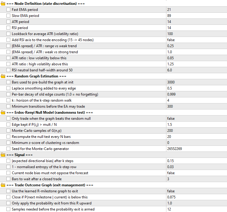
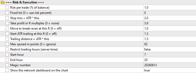
Several settings differ from the code defaults, and they shape how the results should be read. The momentum axis was disabled, so the network used fifteen vertices instead of forty-five. The walk horizon was four bars. The take-profit was 3.9R rather than the default 3.0R. The advance-probability threshold was 0.875 rather than 0.35. Most importantly, the Erdos–Renyi gate was disabled (InpUseNullGate = false), so these results do not measure the effect of the randomness test. We ran two passes that were identical except for InpUseOutcomeGraph. Both used real-tick modelling with 100% history quality.
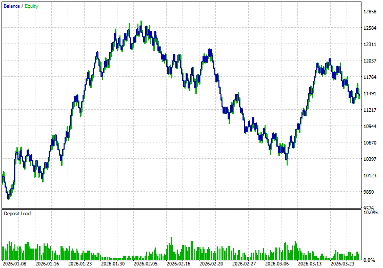
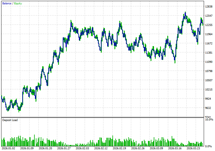
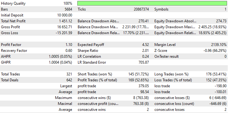
Below is the equity curve and the backtest results:
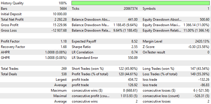
Comparison Table:
| Metric | Graph Exit ON | Graph Exit OFF |
|---|---|---|
| Net profit | $1,451.12 | $2,292.28 |
| Gross profit | $16,652.71 | $15,229.96 |
| Gross loss | -$15,201.59 | -$12,937.68 |
| Profit factor | 1.10 | 1.18 |
| Recovery factor | 0.60 | 1.68 |
| Sharpe ratio | 2.01 | 2.55 |
| Max equity drawdown | $2,405.25 (18.93%) | $1,366.14 (11.00%) |
| Total trades | 321 | 269 |
| Win rate (long) | 53.41% | 43.54% |
| Win rate (short) | 51.72% | 45.90% |
| Avg. profit trade | $98.54 | $126.92 |
| Avg. loss trade | -$100.01 | -$86.83 |
| LR Correlation | 0.24 | 0.74 |
| Tester Z-score (win/loss series) | -0.96 | -0.30 |
The last row is the tester's series Z-score, which measures the dependence between consecutive wins and losses. It is unrelated to the structure z-score used by the null model.
Comparing a fixed 3.9R take-profit with the outcome-graph exit shows that, over this three-month M15 window on XAUUSD, the fixed take-profit performed better on most metrics. It produced higher net profit ($2,292 vs. $1,451), a higher profit factor (1.18 vs. 1.10), and a lower maximum drawdown (11.00% vs. 18.93%). It also showed more consistent equity growth (LR Correlation 0.74 vs. 0.24). The outcome-graph exit achieved a higher win rate on both long and short trades, but its average winning trade was smaller and its average losing trade was larger. On this evidence, the outcome-graph exit did not improve exit management in its tested configuration.
The most likely cause is the threshold itself. With InpMinAdvanceProb set to 0.875, the exit fires whenever the learned chance of reaching the next milestone is below 87.5%. Once twelve samples exist, that condition is almost always true, so the rule behaves much like an early fixed target near 1R to 1.5R. This is consistent with the higher win rate and the smaller average winner. We did not log per-milestone sample counts, so sampling noise remains a possible contributor, but it is a hypothesis rather than a verified finding. The comparison is also not a pure test of exits. Earlier exits free the EA to re-enter sooner, which is why the ON run placed 321 trades against 269, and those different entries also change the loss profile.
Finally, a single three-month test on one instrument and one timeframe cannot establish a durable edge for either configuration. There is no out-of-sample period, walk-forward analysis, or confidence interval here, so we present these results as a demonstration of the mechanics rather than evidence of profitability. A fairer next step is to rerun the comparison with the default threshold, log the sample count at each milestone, extend the history, and validate out of sample.
Conclusion
We started from a limitation that affects almost every system we build, which is the assumption that market structure is fixed. We replaced that assumption with a network whose edges are generated by the market itself and decay when they stop being supported by data. We turned bars into vertices using dimensionless features, turned bar-to-bar movement into weighted edges, and used a k-step random walk to forecast where the process is heading. We then added the piece that turns random graph theory from a modelling idea into a testable one, which is a null model. By generating Erdos–Renyi graphs with the same size and expected density as our market network, we gained a measurable way to ask whether one structural property of our network differs from chance. Finally, we built a second, smaller graph over R-multiple milestones and let it govern exits with probabilities learned from our own trade history.
A reader looking to move beyond a static rule set now has a different set of tools. Instead of tuning thresholds until a curve looks acceptable, we can measure one aspect of the structure an instrument carries, watch that measurement change over time, and optionally refuse to trade when it disappears. The transition matrix is readable, so we can see which market states feed which. The entropy measure tells us when a forecast horizon is too long to mean anything. The outcome graph gives us counted evidence about how far trades travel, and our comparison showed that such evidence still needs careful calibration and an expected-value framing before it can beat a simple fixed target. Each of these is a diagnostic in its own right, and each can be lifted out of this Expert Advisor and dropped into a different system.
There is also a clear path forward from here. The same framework accepts richer vertices, such as swing points, order blocks, and fair value gaps, which would turn the state network into the liquidity network described at the start of this series. The null model can be extended beyond clustering to degree distribution or component structure, and it can be made stricter with a fixed-edge G(n,M) model or a directed, weighted null that respects the Markov structure of the source matrix. The outcome graph can be conditioned on direction and entry state, and given its own decay. The decay factor can itself be adapted, so the network forgets faster during regime change and slower during calm periods. What matters most is the shift in perspective. Once we accept that the graph is generated by a random process, testing our graph against randomness becomes a useful first filter. It is one input among several, not proof of an edge, and every conclusion it supports still has to survive out-of-sample testing.
Warning: All rights to these materials are reserved by MetaQuotes Ltd. Copying or reprinting of these materials in whole or in part is prohibited.
This article was written by a user of the site and reflects their personal views. MetaQuotes Ltd is not responsible for the accuracy of the information presented, nor for any consequences resulting from the use of the solutions, strategies or recommendations described.

 Markov Chains in Trading and Price Forecasting
 Win Rate and Edge Ratio Heatmap by Hour and Symbol in MQL5
 Overcoming Accessibility Problems in MQL5 Trading Tools (Part VII): MetaTrader 5 Model Context Protocol (MCP) the Grand Solution
 Neural Networks in Trading: Robust Trading Signals in Any Market Regime (Attention Modules)

- Free trading apps
- Over 8,000 signals for copying
- Economic news for exploring financial markets
You agree to website policy and terms of use