How to Use Finite Differences for Price Forecasting

Introduction

If I were to ask: What is a trader's main task? The answer is very simple: find a simple and effective tool for market analysis and price forecasting. Finite differences can be used as such a tool.

Finite differences are a numerical method for estimating the derivative of a function using the function's values at discrete points. By using them, a trader can analyze changes in an asset's price over time, identify patterns and trends, and pinpoint potential entry and exit points for positions.

Although finite differences have been known for a very long time, they are not used very often in trading. In this article, we will explore the application of finite differences in trading, starting with the basic concepts and ending with practical examples of their use. The main purpose of this article is to introduce traders to the finite difference method and show how it can be used to make more informed trading decisions.

In this article, we will examine various types of finite differences — forward and central finite differences. Let's discuss their advantages and disadvantages, and explore how finite differences can be used for data smoothing, noise filtering, and forecasting.

Fundamentals of Finite Differences and the Binomial Transform

Finite differences are a numerical method that can be used for interpolating and differentiating functions. This method was described in detail by Brook Taylor in 1715 in his work “Methodus Incrementorum Directa et Inversa”.

The primary purpose of finite differences is to approximate the values of derivatives. The main difference between them is that derivatives are continuous, while finite differences are discrete. Financial time series are also discrete — price values depend on the point size, and changes in those values occur only at specific points in time.

A first-order finite difference is analogous to the ordinary derivative. It is the difference between two successive price values, and calculating it is not particularly difficult.

A second-order difference can be obtained by finding the difference between adjacent first-order finite differences.

Differences of higher orders are obtained in the same way — we take two differences of the previous order and find their difference.

Finite differences can be used for the binomial transform of a time series.

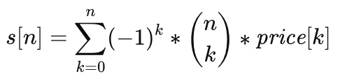
Essentially, this transform is based on several finite differences. In this case, it is assumed that the zeroth-order difference is equal to the value of the time series. The inverse binomial transform reconstructs the original time series. In this form, applying this transform seems pointless.

But let's not jump to conclusions; let's take a moment to recall the Fourier and Hartley transforms. These transforms are based on the decomposition of a time series into a set of wave functions with different frequencies. One of their advantages is the ability to reduce the impact of high-frequency components associated with noise. After that, inverse transforms allow us to construct smoothed time-series models.

The same approach can be applied to the binomial transform. Let's assume that the value of each finite difference consists of two components: signal and noise. Then, after applying the binomial transform, we can try to reduce the effect of noise. That said, we can assume that the effect of noise depends on the order of the finite difference — the higher the order, the stronger the noise.

As an example, I will suppress the noise according to a hyperbolic law: I will reduce first-order differences by a factor of 2, second-order differences by a factor of 3, and so on. By applying the inverse transformation to the resulting values, we obtain a smoothed time series model.

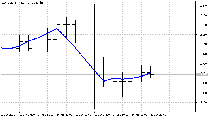
The first success has been achieved. Let's take a look at some other ways to apply finite differences in trading.

Finite Differences and Patterns

A pattern is a consistent, recurring combination of certain factors, events, etc. In technical analysis, patterns refer to any combinations of prices, chart objects, and technical indicators that allow one to predict the future direction of price movement with a high degree of accuracy.

The use of patterns is based on a simple rule: history repeats itself. In other words, when a certain pattern forms on the chart, there is a high probability that the price will move in the same way as it has in similar situations in the past.

Using finite differences allows us to assess the degree of similarity between different segments of a time series. If the finite difference values are the same, then the price dynamics in those segments will be the same. However, the prices themselves may vary. For example, the two most similar sections will look like this.

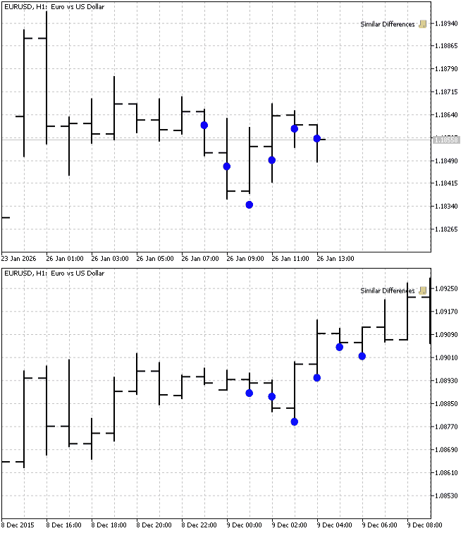
We can use a similar approach to construct price patterns. Let's assume that if the values of the finite differences fall within certain limits, we will consider them similar. We will try to create patterns based on this principle.

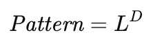
First, we need to specify the number of finite differences, D, and the number of levels, L, that we will distinguish. In that case, the total number of patterns that this model will be able to distinguish can be calculated using the following formula:

In the next step, we need to find the maximum and minimum values of each finite difference in the historical data. Once we know these values, we can calculate the level step size.

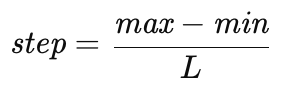
Now that we have the value of the difference, we can calculate its level index, which will range from 0 to L-1.

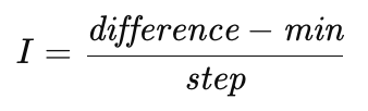
By combining the indices of all the differences, we can obtain the pattern number. To do this, the combination of the indices obtained must be converted to a decimal number.

We've learned how to calculate patterns. Now let's try to apply them in some way. For example, we might assume that future price values somehow mysteriously depend on the current pattern.

First, we need to decide how many bars ahead we will build our forecast. For forecasting, we will use the average of the high and low prices following a given pattern. As a result, we will end up with a statistical forecast that looks like this:

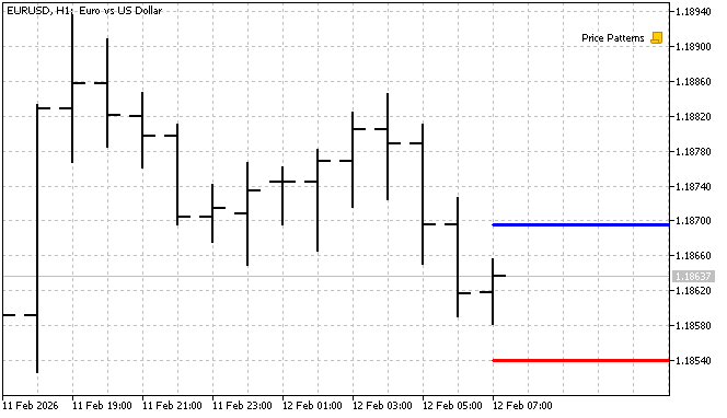
Finite differences can also be used to analyze candlestick patterns. Each candlestick is entirely determined by the OHLC prices. Based on these prices, the following differences can be calculated:

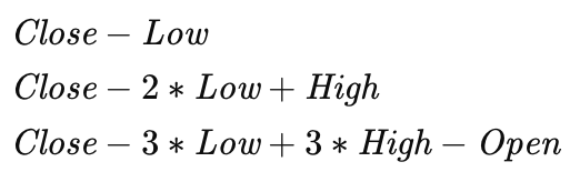
These differences completely determine the candlestick's appearance. The number of patterns for a single candlestick depends solely on the number of levels.

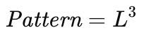
However, such patterns can also be constructed using several candlesticks. In that case, we will first need to identify the patterns for each candlestick individually, and then identify a pattern of those candlestick patterns. In other words, the total number of patterns will depend on the number of levels and candlesticks:

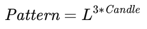
Here is the forecast based on candlestick patterns:

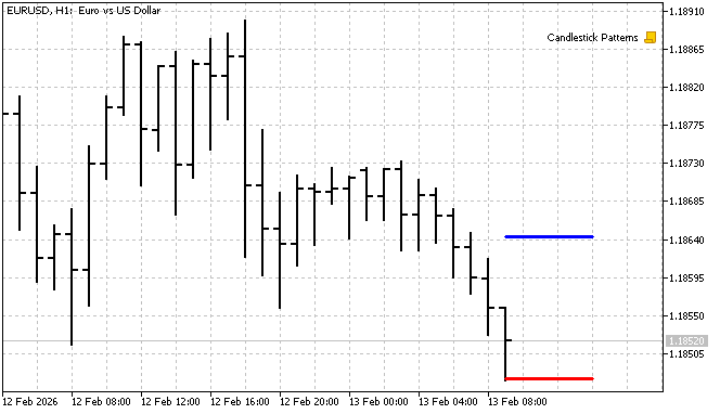
The main challenge in using patterns is determining the optimal number of them. If there are too few of them, the model will be overly generalized and crude. If the number of patterns is too large, the model will become sensitive to noise.

It is also important to note that the difference values are not uniformly distributed, and some patterns may occur more frequently than others. For example, this is what the distribution of first-difference values looks like.

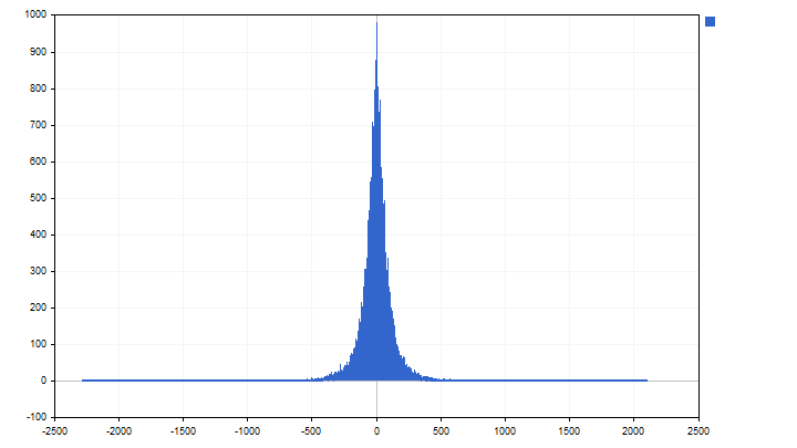
This should be taken into account when making forecasts. The more frequently a pattern occurs in historical data, the higher the level of confidence in the forecast.

Finite Differences and Forecasting

Forecasting in trading generally consists of two stages. Using historical data, a trader looks for patterns in price dynamics and then applies them to the current market situation. However, identifying patterns can take a lot of time and effort. So-called “naive forecasting” does not have this drawback. This forecasting method is based on a simple rule: what has happened in the past will happen again. Let's take a look at how to make naive forecasts.

So, we have the current price, and we want to estimate the future price value. Naive forecasting gives the following answer:

It all looks simple, but this is just the beginning. Let's increase the sampling rate of the time series and obtain a new version of the forecast:

By continuing to increase the sampling rate, we can obtain even more forecasts. In the next step, we can calculate the average of all the individual forecasts obtained. In that case, the final version of the forecast will be as follows:

In other words, a naive forecast based on the time series values is an SMA shifted one bar to the right. Now let's try to build a naive forecast based on price movement. In this forecast, we will assume that the value of the first difference remains unchanged.

We will not be able to obtain such an indicator. More precisely, we can obtain it, but it will be unstable, since one of the main rules has been violated: the absolute values of the indicator's coefficients must be less than 1. Let's increase the sampling rate. In that case, the indicator formula will be as follows:

But an indicator like this will be more stable. We continue increasing the sampling rate, then calculate the average of all forecast versions. As a result, we obtain the indicator formula:

In other words, the next price is equal to the current price plus the average rate of change over the previous N bars. We can apply the same approach to differences of higher orders. For example, the formula for an indicator based on a second-order difference would be as follows:

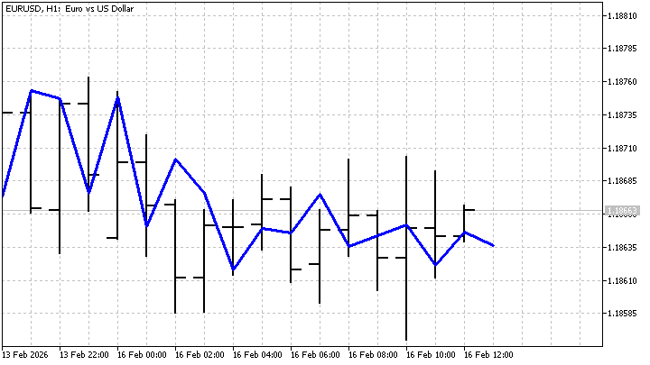
Of course, we can sum the differences with each other. And the indicator itself looks like this:

Finite differences can be used for more than just naive forecasting. These differences can also be used to build an adaptive forecast. Let's take a look at what this forecast is and how to build it. One method of time series analysis is regression. It can be used to identify patterns in price movement. The regression equation is as follows:

But regression has one drawback — to find its coefficients, we need at least N prices. In other words, using this method, we get certain average values, but price movements rarely follow average trends. Price movement can change at any time. Can we detect this change and respond to it?

Let's assume that we already have the regression coefficients. When a new price arrives, we need to adjust them accordingly. In other words, the equation will look like this:

Now let's impose a condition: we need to minimize the forecast error, and at the same time, the change in the regression coefficients must also be minimal. In that case, the change in the coefficients can be found using the following formula:

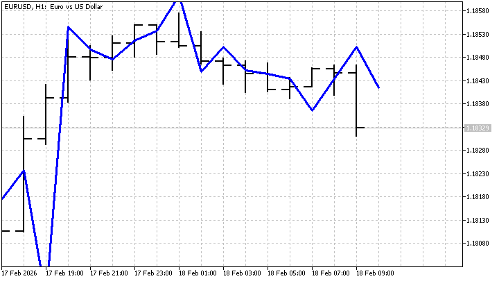
As a result, the regression coefficients will change when each new price arrives, and historical data is needed only to refine the values of these coefficients. Instead of prices, we can use finite differences, and an adaptive indicator based on them will look like this:

Finite differences can also be used to construct probabilistic forecasts. We have the current price and the distribution of first-difference values. Based on this data, we can predict what the next price will be and the probability of that specific value occurring. If we compile statistics on second-order difference values, we can make a forecast based on the last two prices. We will end up with two different forecasts, which we can combine into one. The final probability depends on the probabilities from both distributions. It can be calculated using the following formula:

Using this probability, we can estimate various possible future price values. For example, we can calculate the expected value of the price and its upward and downward movements. And this is what a forecast based on three differences looks like.

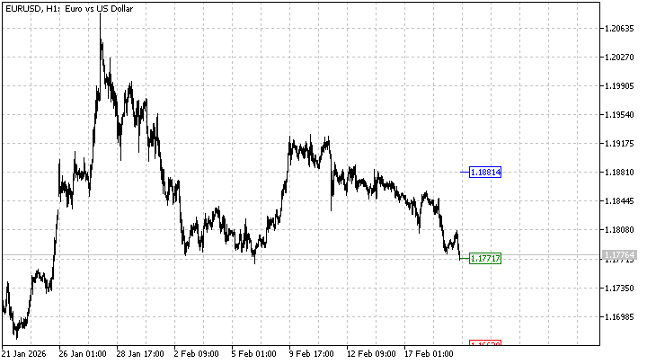
With a probabilistic approach, we can build a wide variety of forecasts. For example, you can assess the most likely channel within which the price will end up. Wherever probability is involved, there can be many different ways to apply it.

Conclusion

In this article, we examined finite differences as a method for market analysis and price forecasting in trading. We reviewed their fundamentals and ways to apply them. In practice, finite differences can be used to solve a wide variety of problems. We have reviewed examples of their use for data smoothing and noise filtering, pattern building, and forecasting.

Although the finite difference method has been known for a long time, its application in trading can offer new approaches to data analysis and help traders make more informed trading decisions. The main challenge lies in selecting the optimal number of differences. Nevertheless, finite differences can be a useful tool in a trader's arsenal.

The following programs were used in preparing this article.

Title	Type	Description
Binomial transform	Indicator	iPeriod — the indicator's period. This same parameter determines the maximum order of the finite differences.
Similar Differences	Script	Difference — the maximum order of finite differences.
Price Patterns	Script	Differences — the maximum order of finite differences. Level — number of levels. Forward — the number of bars ahead to forecast. Pause — how many seconds to display the forecast. The Experts tab displays the forecast values. The image showing the forecast is saved in the Files folder.
Candlestick Patterns	Script	Candle — the number of candlesticks to process.
Naive Forecast	Indicator	Difference — the maximum order of finite differences. iPeriod — the indicator's period.
Adaptive Forecast	Indicator	Difference — the maximum order of finite differences. LearningSpeed — learning rate. The higher this value, the more slowly the coefficients are adjusted.
Probabilistic Forecast	Indicator	There are no parameters. But you can increase the number of differences used.