Walsh Functions in Modern Trading

Introduction

The article focuses on the practical application of Walsh functions in trading. Today's market requires traders not only to analyze historical data, but also to identify patterns that allow them to assess the likely direction of future price movements.

Traditional indicators, oscillators, and chart patterns remain important tools; however, their capabilities are often insufficient for detecting hidden structures in price series. We assume that you have already reviewed the introductory material and understand how Walsh functions are formed.

The purpose of this article is to show how Walsh functions can be applied in trading analysis. The article covers the following:

• the mathematical properties of Walsh functions necessary for their practical application;
• the key advantages and limitations of these functions;
• examples of how they are used to analyze market dynamics, identify trends, and determine potential entry and exit points for trades;
• an illustration of how to develop a trading strategy based on Walsh functions.

The article is intended to help readers develop a systematic understanding of how these functions can expand their analytical toolkit and support trading decision-making.

Properties of Walsh Functions. Advantages and Limitations

Walsh functions form a system of orthogonal functions. They were proposed in 1923 by mathematician J. Walsh as a simpler alternative to the system of trigonometric functions. Orthogonality means that these functions can be used to isolate the most important components that describe the dynamics of a time series.

Walsh functions can be symmetric or antisymmetric about the function's center. This property affects the behavior of the functions: symmetric functions smooth the time series, while antisymmetric functions highlight trend components. The main advantage of Walsh functions is their linearity and computational simplicity. This makes them very useful for analyzing financial time series.

The main drawback of these functions is that the results are difficult to interpret. As an example, let's take a time series with the values: 1, 2, 1, 2. We will apply the first- and second-order Walsh functions to it.

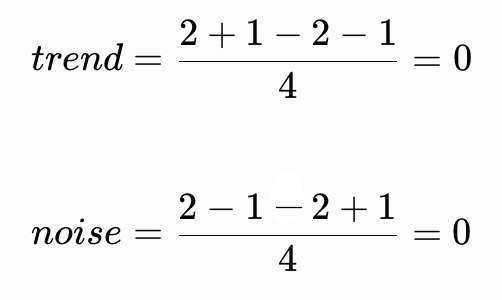
There is no trend, and that much is clear. But I interpreted the even function as noise. And it is not present either. Now I will add a trend component to this time series: 0, 1, 2, 3. Let's perform the calculations again.

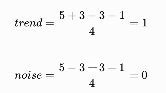
A trend has emerged here, and there is no room for any other interpretation. However, the noise value leads to an ambiguous conclusion: on the one hand, it can be argued that the time series is sufficiently smooth and quite predictable; on the other hand, the value of this function may indicate the presence of a cyclic component.

Another drawback of Walsh functions is their strictly defined period. If I want to build an indicator based on these functions, I won't be able to set its period arbitrarily. It must be a power of 2, which limits the range of applications for these functions.

In trading, Walsh functions can be used to identify patterns in price behavior, forecast future market movements, and make trading decisions. Let's take a look at some of the capabilities of these functions.

Forecasting Using Walsh Functions

Forecasting is important in trading because it allows you to assess future market changes and make informed decisions. Key advantages of predictive models:

• identifying current trends and patterns to predict price movements;
• determining the optimal times to open and close positions and reducing risk;
• developing risk management strategies, such as setting stop-loss and take-profit orders;
• a deep understanding of market conditions and improved analytical and decision-making skills.

Let's take a look at how Walsh functions can be used for forecasting. The zero-order Walsh function is essentially equivalent to the well-known SMA. One of the characteristics of this indicator is that it follows the trend. As the price rises, so does the indicator. When the price falls, the indicator also starts to decline. In other words, when deciding whether to open or close a position, it is helpful for a trader to know what the SMA value will be after a certain number of bars.

The SMA values in the historical data are distributed fairly evenly. Although there are some anomalies in this distribution, they are not significant enough to serve as a basis for making any predictions.

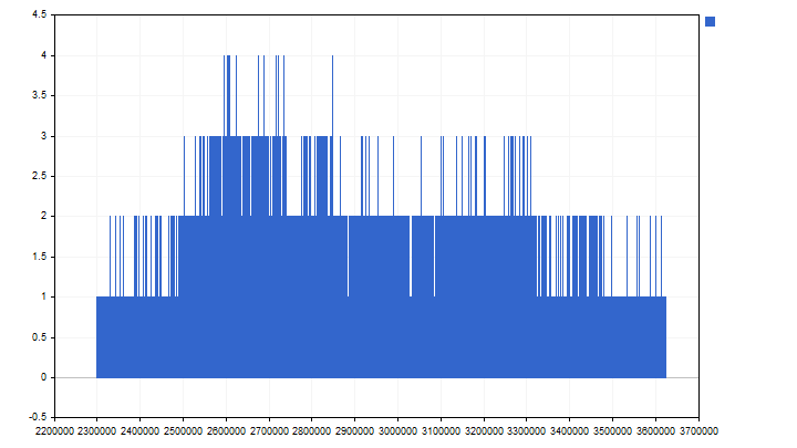
Let's make the approach a little more complex. First, we will gather some statistics on how SMA values can change in general. In other words, we will look for the differences between the current value of this indicator and the value from N bars ago. A first-order Walsh function with a period twice that of the SMA will help us with this. The distribution of the values of this function looks like this.

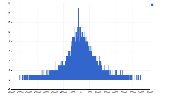
Using this probability density function (PDF), we can predict the future value of the SMA. We know the current value of this indicator. It is reasonable to assume with a high degree of confidence that the difference between the future and current SMA values will follow the distribution obtained. Thus, we will be able to estimate both the future value of the SMA and the probability that it will be exactly that value.

A predictive model can be built based on these PDFs. The algorithm for this model is quite simple. First, we need to calculate the current SMA value. Using the PDF of the first-order Walsh function, find the levels within which the SMA value will be in the future. To do this, we need to add the minimum and maximum PDF values to the current SMA value.

This is where things really get interesting. For all possible values, we need to calculate the probability of their occurrence. To do this, we will need both PDFs. In other words, the probability of observing a specific value depends on the probabilities of both functions.

Knowing these probabilities, we can calculate the expected value of the future SMA value.

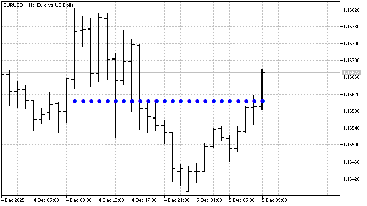
As a result, we will obtain the price level that the SMA is moving toward. On the graph, this forecast looks like this:

Using Walsh functions, it is possible to construct a forecast that is of even greater interest to traders. The first-order function displays the value of the current linear trend. If we add a second-order function with a doubled period, we will be able to estimate future changes in the trend. The forecasting algorithm will remain the same — we collect statistics for each function separately and, based on the current trend, estimate its expected future value.

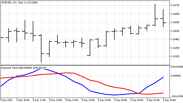
As you can see, the forecasts (the red line) differ quite significantly from the actual values. However, this discrepancy provides insight into the overall market situation. A large difference may indicate high volatility or significant changes in the market. In any case, it is important to remember that forecasting is not always accurate (more often than not, it is inaccurate), and traders need to take all risks and uncertainties into account when making decisions.

Modifying the Classics

As I mentioned earlier, one of the limitations of Walsh functions is their strictly defined period. If, for example, we decide to construct a system of third-order functions, their period will be 8. But this restriction can be easily circumvented. All Walsh functions are constructed from periodic functions, so we can increase their period by any integer factor. This capability will allow us to create more flexible indicators.

Another property of Walsh functions is that they are windowed. On the one hand, this is good — we can observe the evolution of price throughout the entire window. On the other hand, however, some traders may not like this property. This is because the indicator's value on each bar will depend on both past and future prices within the window. Simply put, the indicator repaints its past values. We can also eliminate this behavior — for each bar, we will calculate the indicator's value only once, when the bar appears.

As a result of these changes, we can obtain a rather distinctive indicator. The odd functions should make it follow trends, while the even functions should smooth out its values. In addition, we can add a market-noise suppression feature to this indicator. This will provide additional smoothing.

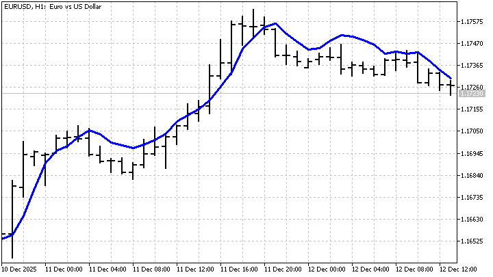
As you can see, the indicator does its job — it tracks the price and looks fairly smooth. If we could predict its value, we could come up with a pretty good trading strategy.

You might naturally wonder: am I confusing cause and effect? After all, this indicator is the effect, while price is the cause. The indicator follows the price, not the other way around. Imagine that we can observe the path of a drunken sailor with a dog. We do not know: maybe the sailor dragged the dog along with him, or maybe the dog went off on its own business, and the sailor had to follow it. Be that as it may, it is easier for us to predict the sailor's path — it is simply chaotic. But predicting the dog's path is more difficult — the dog's own chaos is added to the sailor's chaos. In this case, the indicator is the sailor, and prices are his dog. And it is easier for us to follow the sailor than the prices. But how do we build such a forecast? We do not know that yet.

We can estimate the length of the leash by subtracting the indicator value from the price. But it is much more interesting to find out how Walsh functions assess the current price movement. If we discard the zero-order function, we will end up with an oscillator that indicates the strength and direction of the trend.

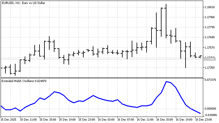
As you can see, the resulting oscillator handles this task well.

Developing a Trading Strategy

A trading strategy is a set of specific rules that govern trading operations. These rules can vary widely, ranging from the simplest — such as an SMA crossover — to the most complex, involving AI and other mysterious things. Let's try developing our own strategy using Walsh functions.

So, we have an indicator whose movement we would like to predict. However, this movement depends on the price value and is random. Markov chains can be used to predict such processes. They were named after A. Markov, who introduced them in 1906 in his article “Extension of the Law of Large Numbers to Dependent Quantities.” These chains consist of a sequence of random events. In this case, the probability of an event occurring depends solely on the state reached in the previous event.

For example, we distinguish between two states of the indicator based on the direction of its movement — up or down. Using historical data, we can track changes in the indicator's state and calculate the probability of a transition from one state to another. It is easier to represent these probabilities as a matrix.

	up	down
up	0.8	0.2
down	0.3	0.7

The rows show the current states, and the columns show the future states. But this matrix only shows us the next step. To make a two-step forecast, we need to multiply this matrix by itself.

We can continue forecasting further ahead. To do this, we need to multiply the resulting matrices by the original one. For example, this is what the transition probabilities over three steps will look like.

Now let's try building such a chain in practice. The indicator's values can be used as its states. First, we need to specify the number of states that the chain will distinguish and find the minimum and maximum values of the indicator over the entire history. After that, we can determine the state change step.

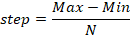
Knowing this step, we can determine which state the indicator was in at any given moment.

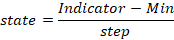
Next, we need to create a square matrix whose size is equal to the number of states. In this matrix, we will store statistics on changes in the indicator's states. Suppose that the current and next states of the indicator have indices I and J, respectively; in that case, we need to increment the value of the matrix element with those indices by 1.

Using these statistics, we can derive a probability matrix. To do this, we first need to find the sum of all elements in each row, and then divide each element in that row by this sum.

A trading strategy could be as follows. Using a probability matrix, I can forecast the indicator’s future states; at each step of the forecast, I will select the most probable state; I will open positions based on the direction and strength of the forecast; and I will close positions using a simple trailing stop. The result of applying this strategy might look like this:

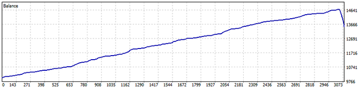
The use of Markov chains complicates the strategy. The properties of a chain depend on the number of states of the chain. If there are too few or too many states in the chain, the chain will lose its ability to learn and make predictions. Therefore, selecting the optimal number of states becomes a very important task for a trader. Despite this, Markov chains are a good mathematical model that can be used in trading.

Conclusion

In this article, we explored the potential applications of Walsh functions in trading. Despite some limitations and drawbacks, these functions can be used to forecast market trends and develop trading strategies. Although the accuracy of forecasts cannot be guaranteed, analyzing the discrepancy between forecasts and actual values can provide additional insight into market conditions. I would like to emphasize once again that Walsh functions can be a valuable tool in a trader's arsenal, and their potential has not yet been fully explored.

The following software programs were used in writing this article.

Name	Type	Description
SMA Trend PDF	script	The script constructs the distribution for the SMA and the trend. Type - indicator type; iPeriod - SMA period.
Expected SMA	indicator	SMA forecast PeriodSMA - indicator period; NumBar - the bar index for which the forecast is being generated.
Expected Trend	indicator	The indicator displays the current and forecast trend values. HalfPeriod - half-period of the trend; BarsHistory - the bar from which to start drawing the lines.
Extended Walsh Functions	indicator	An indicator based on modified Walsh functions. P - the order of the system of functions; N - the period multiplier of the functions; Noise - noise suppression level.
Extended Walsh Oscillator	indicator	An oscillator based on modified Walsh functions.
EA Walsh Markov	Expert Advisor (EA)	An Expert Advisor (EA) based on Walsh functions and Markov chains. State - number of states; Forward - the number of bars ahead for which the forecast is made; MinLvl - minimum state change required to open positions; Profit - the position profit required to trigger a trailing stop.