Developing a Trading Strategy: Using a Volume-Bound Approach

Introduction: The Overlooked Power of Volume

Price movement in financial markets does not occur in isolation. Behind every shift—whether explosive or subtle—lies the force that drives it: volume. However, in the world of technical analysis, price often takes center stage. Traders carefully map out support, resistance, and chart patterns, but often overlook the key force that actually drives these price movements. Volume is the engine of the market, and understanding its language is key to transitioning from a passive chart-watcher to an informed, strategic trader.

In this article, we introduce a mathematical approach to transform raw, unbounded volume data into a bounded form—what we call the Volume Boundary. We then explore how this processed volume can form the foundation of a trading strategy. The goal is to make volume easier to interpret, more consistent across market conditions, and directly usable within algorithmic or discretionary trading systems.

Understanding Volume: The Market's Pulse

At its core, volume is simply the number of trades or contracts exchanged during a specific period, whether it be 5 minutes, 1 hour, or a full trading day. It acts as a measure of activity and certainty, answering the "why" behind price action.

• High Volume: A price movement accompanied by high volume is considered strong and likely to continue. It signifies broad market participation, giving the move credibility and force. For example, a stock breaking out of a consolidation pattern on high volume is a much stronger signal than the same breakout on low volume.

• Low Volume: Conversely, a price move on low volume is viewed as weak and potentially unreliable. It suggests a lack of consensus and may reverse quickly, as it doesn't have the support of the broader market participant base.

While numerous indicators like the Market Facilitation Index (MFI), On-Balance Volume (OBV), and the Accumulation/Distribution attempt to incorporate volume, they often present derived or cumulative values that can be difficult to standardize. Our goal is to work with volume more directly by first constraining its infinite nature into a predictable, bounded range.

By integrating volume into analysis, traders shift from simply observing what the price is doing to understanding why it is happening and how strong the move is.

A Crucial Distinction: Real Volume vs. Tick Volume

It is essential to recognize that the "volume" data available to traders is not uniform across all markets.

• Stock Market (Real Volume): In centralized exchanges like the NYSE or NASDAQ, volume is precise and definitive. It represents the actual number of shares traded. If 5 million shares of Microsoft are traded in a day, the daily volume is 5 million. This data is reported in real-time and is highly accurate.

• Forex Market (Tick Volume): The foreign exchange market is decentralized, with no single entity reporting total volume. Instead, Forex brokers provide tick volume, which is a proxy for actual trading activity. Tick volume measures the number of times the price changes (or "ticks") during a given period. The underlying logic is sound: a high number of price changes typically implies a high level of trading activity and genuine volume. 

Despite this difference, tick volume has been shown to correlate strongly with actual traded volume in decentralized markets, and is widely accepted for volume analysis in Forex. For the purposes of this study, we will use tick volume as the foundational input for our Volume Boundary indicator.

The Mathematical Foundation: Formulating the Volume Boundary

To build the Volume Boundary indicator, we use tick volume and transform it mathematically onto a new, bounded scale. Raw volume (or tick volume) is unbounded—it can increase indefinitely—making it difficult to use directly for thresholds or oscillators. To make volume behavior more interpretable, we perform two key operations:

1. Transform the raw volume using a scaling function (normalization or logarithmic transformation).

2. Pass the scaled volume through a nonlinear smoothing function to bound it within a fixed range.

Normalized Transformation: This method scales the volume based on its recent statistical properties, making it mean-reverting. 

Logarithmic Transformation: This method reduces the impact of extremely large volume values by compressing them, while slightly expanding smaller values. It’s especially useful in markets where volume often spikes irregularly, helping create a more balanced and readable scale. 

Where:

• t  = the scaled volume value
• m  = a scaling factor for sensitivity adjustment
• AvgVol  = the simple moving average of volume over a defined period
• StdVol  = the standard deviation of volume over the same period
• Volume  = the current volume

While these transformations standardize the data, the output ( t ) remains technically boundless. The next, crucial step is to pass this scaled value through a smoothing function that constrains it within a fixed, predictable range.

The Smoothing Function: Creating the Boundary

After transformation, the scaled volume is passed into a smoothing function to force it into a fixed range. This makes the value oscillatory, smooth, and suitable for thresholds in an indicator.

1. The Butterfly Curve Function

The x-component of the butterfly curve is utilized. This nonlinear, cyclical function is applied to the transformed volume  t  to bound it within a range of approximately +3.0 to -3.0. Its complex wave-like nature allows it to capture nuances in volume activity. The function is expressed as:

f(t) = sin(t) × expr

Where:  expr = e^(cos(t)) − 2cos(4t) − ( sin(t/12) )^5

The butterfly curve's repeating, bounded pattern is ideal for identifying cyclical extremes in volume-based momentum.

For the butterfly curve visualization and details-->:  https://www.mql5.com/en/articles/20113

      2. The Triple Sine Function

A simpler yet effective alternative, the triple sine function bounds the scaled volume within a strict range of +1 to -1. This creates a classic oscillator look, familiar to users of RSI or Stochastics. The function is:

f(t) = ( sin(t) )^3

This function provides a clean, normalized output where extremes are easily identifiable as the indicator approaches the +1 or -1 boundaries.

For the triple sine function plot and details, read here: https://www.mql5.com/en/articles/20220

Constructing the Volume Boundary Indicator

To compute the normalized volume, we need the average and standard deviation of volume over a chosen period. The trading platform must calculate the two key statistical components for each new bar.

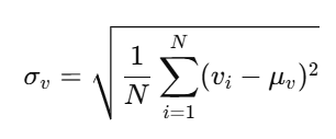
Standard Deviation of Volume is given as: 

Simplifying, we obtain the computational form commonly used in indicators: 

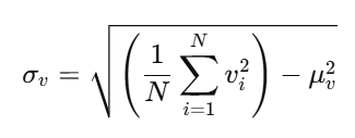
Where: 

• σ = standard deviation
• N = number of volume samples
• μ = simple average volume
• v = individual volume value

Summarizing the workflow:

1. Compute AvgVol and StdVol.
2. Transform volume using either normalization or logarithmic scaling.
3. Pass the transformed value into a smoothing function
- Butterfly curve  
- Triple sine curve
4. Output the result as the Volume Boundary Indicator.

For normalization:

• volume → scaled value → smoothing function → bounded output

For logarithmic scaling:

• volume → log(volume) → smoothing function → bounded output

Indicator Code Structure

With the mathematical foundation established, we now turn our attention to implementing the Volume Boundary Indicator on the MetaTrader 5 platform. This section explains the core components of the indicator, the key parameters available to the user, and how the indicator internally computes volume statistics and scaled values.

input int VolumePeriod = 20;                    // Period for volume average and std dev
input double ScaleFactor = 1.0;                 // Scaling factor (m)
input ifcn InputMethod = 1;                     // Input method
input sfcn SmoothingMethod = 1;                 // Smoothing method

The indicator is designed with flexibility in mind, allowing traders to tailor its behavior to their specific strategy and market. This is achieved through external input parameters:

• VolumePeriod defines how many bars are used to calculate the average and standard deviation of volume.
• ScaleFactor (m) applies a multiplier to the transformed volume values.
• InputMethod allows selection between normalized transformation and logarithmic transformation.
• SmoothingMethod lets the user choose between the Butterfly Curve and Triple Sine smoothing functions.

   // Set indicator range based on smoothing method
   if(SmoothingMethod == ButterflyCurve)
   {
      IndicatorSetDouble(INDICATOR_MINIMUM, -3.2);
      IndicatorSetDouble(INDICATOR_MAXIMUM, 3.2);
   }
   else
   {
      IndicatorSetDouble(INDICATOR_MINIMUM, -1.2);
      IndicatorSetDouble(INDICATOR_MAXIMUM, 1.2);
   }

A critical step in the initialization is setting the visual bounds of the indicator window. This is dynamically configured based on the user's chosen smoothing function to ensure the histogram is displayed clearly without any data clipping. 

• Butterfly Curve: The bounds are set to -3.2 and +3.2, accommodating the wider natural range of this function's output.

• Triple Sine: The bounds are set to -1.2 and +1.2, perfectly framing the oscillator's typical range of -1 to +1 with a small margin.

This dynamic adjustment guarantees that the plotted data fits optimally within the oscillator window, enhancing visual clarity and interpretation.

//+------------------------------------------------------------------+
//| Calculate average volume and standard deviation                  |
//+------------------------------------------------------------------+
void CalculateVolumeStats(int pos, int rates_total, const long &tick_volume[])
{
   double sum = 0.0;
   double sumSq = 0.0;
   int count = 0;
   
   for(int i = pos; i < pos + VolumePeriod && i < rates_total; i++)
   {
      double volume_val = (double)tick_volume[i];
      sum += volume_val;
      sumSq += volume_val * volume_val;
      count++;
   }
   
   if(count > 0)
   {
      AvgVolBuffer[pos] = sum / count;
      double variance = (sumSq / count) - (AvgVolBuffer[pos] * AvgVolBuffer[pos]);
      StdVolBuffer[pos] = MathSqrt(MathMax(variance, 0));
   }
   else
   {
      AvgVolBuffer[pos] = 0;
      StdVolBuffer[pos] = 1;
   }
}

The  CalculateVolumeStats()  function is the computational workhorse that derives the essential statistical baseline from the raw tick volume data.

Key steps:

1. The function loops through the specified  VolumePeriod  to compute the sum of volumes and the sum of their squares.
2. It then calculates the simple average ( AvgVolBuffer ).
3. Using the computed average, it derives the variance and, subsequently, the standard deviation ( StdVolBuffer ). The  MathMax(variance, 0)  ensures the variance is never negative, a crucial step for numerical stability.
4. These values are stored in indicator buffers for use in the subsequent transformation step.

//+------------------------------------------------------------------+
//| Calculate scaled input t                                         |
//+------------------------------------------------------------------+
double CalculateInputT(int pos, const long &tick_volume[])
{
   double currentVolume = (double)tick_volume[pos];
   double t = 0;
   
   if(InputMethod == scaledMethod)
   {
      if(StdVolBuffer[pos] != 0)
         t = ScaleFactor * (currentVolume - AvgVolBuffer[pos]) / StdVolBuffer[pos];
      else
         t = 0;
   }
   else // logMethod
   {
      if(currentVolume > 0)
         t = ScaleFactor * MathLog(currentVolume);
      else
         t = 0;
   }
   
   return t;
}

The  CalculateInputT()  function is where the raw volume is scaled into the standardized value  t , ready for the final bounding operation.

Logic flow:

• The function first fetches the current bar's tick volume.

• If the Normalized (scaled) Method is selected, it calculates  t  using the formula:
  t = m * (Volume - AvgVol) / StdVol . This measures how many standard deviations the current volume is from its recent average.

• If the Logarithmic Method is chosen, it computes  t  as:
  t = m * log(Volume) , which compresses the volume scale and handles large value ranges more effectively.

• The resulting value  t  is returned and will later be passed to the selected smoothing function (Butterfly or Triple Sine) to generate the final bounded indicator value.

   for(int i = limit; i >= 0; i--)
   {
      // Calculate volume statistics
      CalculateVolumeStats(i, rates_total, tick_volume);
      
      // Calculate scaled input t
      double t = CalculateInputT(i, tick_volume);
      
      // Apply smoothing function
      if(SmoothingMethod == ButterflyCurve)
      {
         OscillatorBuffer[i] = ButterflyMethod(t);
      }
      else // Triple sine method
      {
         OscillatorBuffer[i] = TripleSineMethod(t);
      }
   }

This section of the indicator performs the core computation for the Volume Boundary Oscillator. The loop processes each bar from the most recent backward, ensuring that the indicator updates efficiently and accurately.

1. Volume statistics are computed first
   The function CalculateVolumeStats() determines the average and standard deviation for the chosen lookback period. These values are essential for normalized transformation.

2. The scaled input value t is computed
   Using CalculateInputT() , the code transforms the raw volume into a scaled form—either through normalization or logarithmic transformation, depending on the user’s selection.

3. The smoothing function is applied

   • If the Butterfly Curve is selected, the scaled value t is passed to ButterflyMethod(t).

   • If Triple Sine is selected, TripleSineMethod(t) is used instead.

4. Result stored in the oscillator buffer
   The computed output is placed into OscillatorBuffer[i] , which is then plotted on the chart as the final bounded volume oscillator.

In essence, this loop forms the engine of the indicator—transforming raw volume into a mathematically bounded oscillator using the selected smoothing method.

Demonstrating How the Volume Bound Oscillator Works

In this section, we examine how the Volume Bound Oscillator (VBO) behaves visually on the chart under the two available input transformation methods: Normalized Transformation and Logarithmic Transformation. These examples help illustrate how the indicator reacts to changes in market activity and how the smoothing functions influence its output.

Using the Normalized Transformation:

When the normalized method is applied (Figure 1), the oscillator fluctuates freely across both positive and negative regions. Because this method adjusts volume relative to its mean and standard deviation, the VBO becomes highly responsive to shifts in volatility and trading activity. This behavior remains consistent across all timeframes and for both smoothing functions—the Butterfly Curve and Triple Sine. 

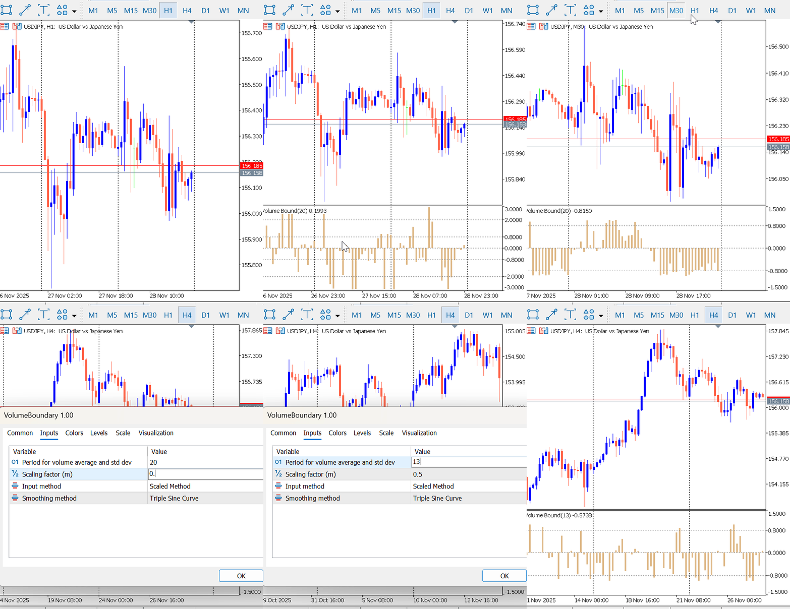
Figure 1 : VBO Normalized Transformation

Using the Logarithm Transformation:

When the logarithmic transformation is selected (Figure 2), the indicator also oscillates between positive and negative levels. However, the behavior differs from the normalized method. The oscillator may remain on one side of the zero line for extended periods. This occurs when raw volume values show only slight variation, causing the log-scaled output to change slowly because the logarithm function compresses the scale of the raw volume data.

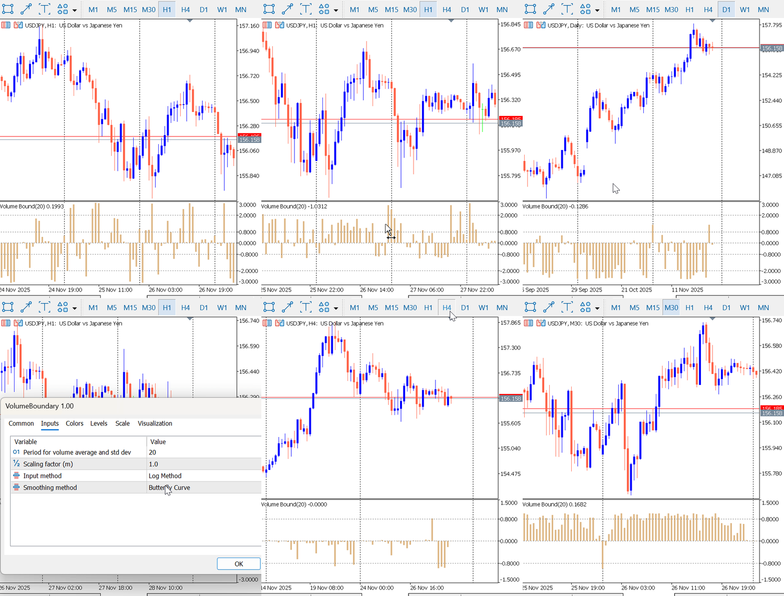
Figure 2: VBO Logarithmic Transformation

Developing Volume Bound Expert Advisor (VBO-EA)

With the Volume Bound Oscillator fully developed, we now extend its application by constructing a trading strategy and Expert Advisor (EA) that uses the indicator to generate actionable buy and sell signals. The VBO can produce signals in several ways, such as:

• Threshold Method – reacting to predefined upper and lower boundary levels
• Histogram Slope Method – analysing increasing or decreasing oscillator bars
• Zero-Line Crossing Method – detecting changes in market momentum

In this article, we demonstrate the threshold-based approach, enhanced with basic price-action confirmation.

Trading Strategy: Threshold & Price Action Confirmation

This approach requires the VBO to breach a predefined threshold level, confirmed by the direction of the price candle itself. This dual-layered filter helps ensure that the volume signal is accompanied by a corresponding price move, increasing the trade's validity.

Entry Criteria

Buy Signal:

A buy trade is opened when both conditions below are met:

1. The last closed candle is bullish (Close > Open)
2. The VBO signal crosses above or below a specified threshold level

The threshold level can be positive or negative depending on the smoothing method used and the trader’s settings.

Sell Signal:

A sell trade is opened when:

1. The last closed candle is bearish (Close < Open)
2. The VBO signal crosses above or below the selected threshold

This combines volume-based confirmation with directional price behavior.

Exit Rules

Each trade will be managed with predefined Take Profit (TP) and Stop Loss (SL) levels. These can be set as fixed pip values or percentages of account equity. We use fixed pips value to exit our positions.

Multiple Entry Logic

The strategy allows two entries in the same direction, but with an alternating threshold to avoid clustering trades at the same signal.

The rules are:

• If the first entry occurs at a positive threshold,
  then the second entry must occur at a negative threshold (and vice versa).

• Only the threshold condition is required for the second entry—price action confirmation is not needed.

This alternating-threshold approach helps diversify entries and avoids over-concentration on a single momentum burst.

Example:

• First Buy Entry: Triggered at a negative threshold, supported by price-action confirmation
• Second Buy Entry: Triggered at a positive threshold, without requiring price-action confirmation

This structure ensures that follow-up entries occur under different volume conditions, improving balance and reducing redundancy.

Demonstrating the VBO Expert Advisor

The VBO-EA provides a flexible set of user-configurable inputs that allow traders to tailor the strategy to their preferred market conditions and risk profile. These inputs can also be optimized within MetaTrader 5 to enhance performance and identify the most effective parameter combinations.

The EA exposes a range of configurable settings, including:

• Indicator parameters(transformation method, smoothing method, scale factor, volume period)
• Trading parameters such as lot size
• Threshold levels used for Buy and Sell signals
• Take Profit and Stop Loss valuesfor managing risk

These settings, illustrated in Figure 3, give traders full control over how the VBO-EA interprets volume behavior and executes trades.

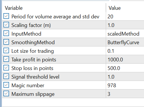
Figure 3: VBO-EA Input

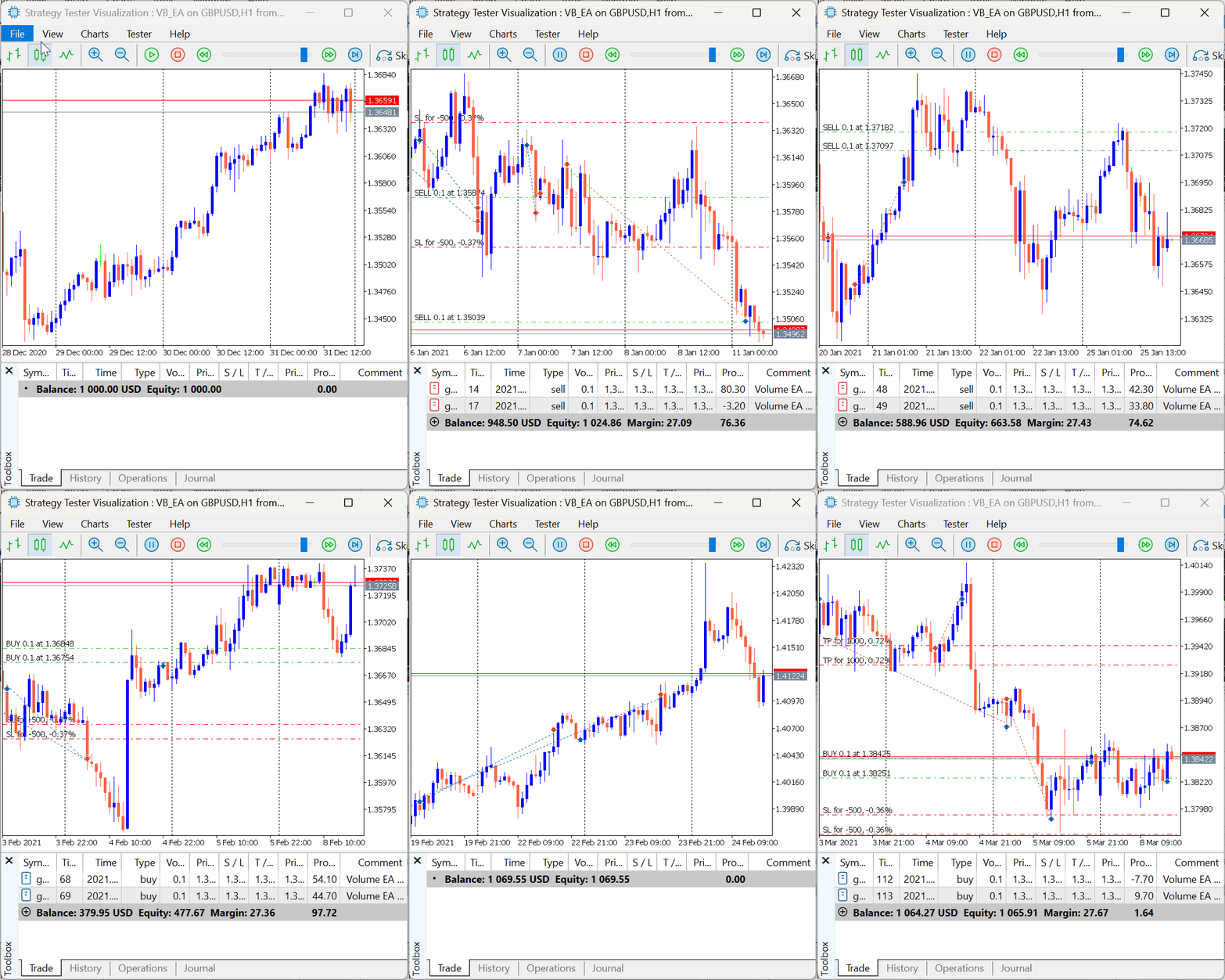
Figure 4: VBO EA Demonstration

Conclusion

This article has introduced the Volume Boundary Oscillator (VBO), a new approach that transforms raw market volume into a bounded and interpretable signal using mathematical functions such as the Butterfly Curve and Triple Sine. By converting unbounded volume into a controlled oscillatory form, the VBO provides a clearer picture of market participation, momentum, and activity shifts across different timeframes.

We further demonstrated how the Volume Bound Expert Advisor (VBO-EA) converts this indicator into a complete trading framework. From volume transformation and smoothing to threshold-based entries, price action confirmation, and structured multiple-entry logic, the EA showcases how mathematical processing of volume can support automated trade execution and systematic decision-making.

This study highlights the value of reimagining traditional market elements—such as volume—through mathematical structures to gain fresh perspectives and improve trading clarity.

In our next work, we will test other strategies and in combination with different indicators to identify the most effective pairings under various financial instruments. Until then, happy trading.

File Name	Description
VolumeBoundary.mq5	This file contains the indicator, which is displayed in a separate chart window. It processes and visualizes the bounded volume data, allowing traders to observe the oscillator’s behavior independently from the main price chart.
VB_EA.mq5	This file contains the Expert Advisor responsible for executing automated trading decisions. It integrates the logic of the Volume Boundary Oscillator, processes incoming signals, and manages trade entries and exits according to the defined strategy rules.