Biological neuron for forecasting financial time series

Modern trading is undergoing a revolution. Neural networks, genetic algorithms, deep learning — all these tools produce impressive results, but often suffer from one significant drawback: they are too "mechanical" and unable to capture the subtle nature of market fluctuations, which are essentially the result of the collective behavior of living market participants.

In this context, the use of biologically plausible neural models becomes particularly relevant. Instead of creating abstract mathematical constructs, we turned to the most advanced computer in the observable part of the Universe - the human brain. Our research group has developed a unique system based on the Hodgkin-Huxley model that simulates not only the functionality but also the physical nature of neural processes.

The Nobel Prize-winning Hodgkin-Huxley model describes the mechanism of generation and propagation of nerve impulses at the cellular level. But why might this particular model be the key to understanding financial markets? The answer lies in the striking analogy between the spread of nerve impulses in the brain and the spread of information in markets. Just as neurons exchange electrical signals through synaptic connections, market participants exchange information through trading transactions.

The innovation of our approach lies in adding a plasma-like component to the classical model. We view a neural network as a dynamic system immersed in the "plasma" of market information, where each neuron can influence the behavior of other neurons not only through direct connections, but also through the electromagnetic fields it creates. This allows the system to capture subtle correlations and relationships that go unnoticed by traditional algorithms.

In this article, we will take a detailed look at the system architecture, its operating principles, and the results of practical application on various financial instruments. We will show how a biologically inspired approach can offer a new perspective on the problem of financial time series forecasting and open new horizons in the field of algorithmic trading.

Hodgkin-Huxley model: When biology meets finance

Imagine a neuron — an amazing cell able to handle and transmit information through electrical impulses. It was this fundamental unit of the brain that Alan Hodgkin and Andrew Huxley described in their groundbreaking work, for which they later received the Nobel Prize. Their model was a real breakthrough in neuroscience, and now imagine that this same model can help us understand and predict the movements of financial markets.

At the very heart of the model lies a mathematical description of how a neuron generates electrical impulses. Just as traders react to incoming market information, a neuron reacts to incoming signals by creating its own unique pattern of activity. Let's take a look at the code that describes this amazing process:

class HodgkinHuxleyNeuron:
    def __init__(self):
        self.V = -65.0  # Initial resting potential
        self.m = 0.05   # Activation of sodium channels
        self.h = 0.6    # Inactivation of sodium channels
        self.n = 0.32   # Activation of potassium channels
        self.last_spike_time = float('-inf')

Ion dance: How neurons make decisions

The most striking thing about the Hodgkin-Huxley model is its description of how ions "dance" across the neuron membrane. Sodium and potassium, the two key players in this molecular ballet, move through special channels, creating an electrical potential. This is very similar to how order flows create price movement in the market. In our trading system, we use this analogy by converting market data into ionic currents:

def ion_currents(self, V):
    I_Na = self.g_Na * (self.m ** 3) * self.h * (V - self.E_Na)  # Sodium current
    I_K = self.g_K * (self.n ** 4) * (V - self.E_K)             # Potassium current
    I_L = self.g_L * (V - self.E_L)                             # Leakage current
    return I_Na, I_K, I_L

Plasma influence: A new look at neural networks

We went beyond the classical model and added the concept of a plasma-like environment. Imagine that neurons are not simply connected by synapses, but are immersed in the "information plasma" of the market. Each neuron spike creates a wave of influence that fades over time, just like a piece of news on the market gradually loses its impact on the price:

def plasma_influence(self, current_time):
    time_since_spike = current_time - self.last_spike_time
    influence = self.plasma_strength * np.exp(-time_since_spike / self.plasma_decay)
    return influence * self.get_market_correlation()

Learning through Time: The STDP Mechanism

Perhaps the most exciting part of our system is the learning mechanism based on the temporal dependence between neuronal spikes (STDP). Just as a trader learns from experience, our neurons adjust the strength of their connections depending on how successfully they predicted market movements:

def update_synaptic_weights(self, pre_spike, post_spike, weight):
    delta_t = post_spike - pre_spike
    if delta_t > 0:
        return weight * (1 + self.A_plus * np.exp(-delta_t / self.tau_plus))
    else:
        return weight * (1 - self.A_minus * np.exp(delta_t / self.tau_minus))

This biologically inspired architecture allows our system to not just handle market data, but to "feel" the market like an experienced trader. Each neuron becomes a mini-expert on its own aspect of market dynamics, and their collective work creates remarkably accurate forecasts.

System architecture: from biology to trading decisions

Imagine the brain of a trader analyzing the market. Thousands of neurons process information about prices, volumes, indicators, and news. It is this natural architecture that we have recreated in our system, adding to it the unique properties of plasma and electromagnetic interactions.

Eyes of the system: Input data structure

Just as the human brain receives information through the senses, our system collects and handles a multitude of market signals. Every tick, every price movement is converted into neural impulses. Let's take a look at the data preprocessing code:

class MarketFeatures:
    def __init__(self, window_size=20):
        self.window_size = window_size
        self.scaler = StandardScaler()
        
    def add_price(self, price: float, ohlc_data: pd.DataFrame) -> Dict[str, float]:
        features = {}
        
        # Technical indicators
        features['sma_10'] = self._calculate_sma(ohlc_data['close'], window=10)
        features['ema_20'] = self._calculate_ema(ohlc_data['close'], window=20)
        features['rsi'] = self._calculate_rsi(ohlc_data['close'], window=14)
        
        # Volumetric characteristics
        features['volume_sma'] = self._calculate_sma(ohlc_data['tick_volume'], window=10)
        
        # Temporal patterns
        features['hour'] = ohlc_data.index[-1].hour
        features['day_of_week'] = ohlc_data.index[-1].dayofweek
        
        return self.scaler.fit_transform(np.array(list(features.values())).reshape(1, -1))

Neural network: A bridge between biology and mathematics

At the heart of our system is a hybrid architecture that combines classical neural networks with the biologically plausible Hodgkin-Huxley model. Each neuron here is not just a mathematical function, but a small living system:

class BioTradingModel(nn.Module):
    def __init__(self, input_size, hidden_size, output_size):
        super(BioTradingModel, self).__init__()
        self.layers = nn.ModuleList([
            nn.Linear(input_size, hidden_size),
            nn.Tanh(),
            nn.Linear(hidden_size, hidden_size),
            nn.Tanh(),
            nn.Linear(hidden_size, output_size)
        ])
        
        # Biological neurons
        self.bio_neurons = [HodgkinHuxleyNeuron() for _ in range(hidden_size)]
        self.plasma_field = PlasmaField(hidden_size)

Plasma field: A new dimension of neural interactions

The uniqueness of our system lies in the plasma-like environment in which the neurons are immersed. Just as electromagnetic fields permeate space, our plasma creates an additional level of interaction between neurons:

class PlasmaField:
    def __init__(self, size):
        self.field_strength = np.zeros(size)
        self.decay_rate = 0.95
        
    def update(self, neuron_activities):
        # Update the field based on neuron activity
        self.field_strength = self.field_strength * self.decay_rate
        self.field_strength += neuron_activities
        
    def get_influence(self, neuron_index):
        # Calculate the influence of a field on a specific neuron
        return np.sum(self.field_strength * np.exp(-self.distance_matrix[neuron_index]))

Learning mechanism: Dance of neurons and plasma

In our system, training occurs on several levels simultaneously. Classical gradient descent is combined with biological STDP and plasma dynamics:

def train_step(self, inputs, target):
    # Straight pass
    predictions = self.forward(inputs)
    loss = self.criterion(predictions, target)
    
    # Backpropagation
    self.optimizer.zero_grad()
    loss.backward()
    
    # Biological education
    for i, neuron in enumerate(self.bio_neurons):
        # STDP update
        neuron.update_weights(self.last_spike_times)
        
        # Plasma modulation
        plasma_influence = self.plasma_field.get_influence(i)
        neuron.modulate_weights(plasma_influence)
    
    self.optimizer.step()
    return loss.item()

This multi-layered architecture allows the system to capture not only obvious patterns in the data, but also subtle, barely noticeable relationships between different aspects of market dynamics. Each component of the system plays its own unique role, and their synergy creates something greater than the sum of its parts – a true artificial brain for analyzing financial markets.

Technical indicators: the digital senses of our system

If we imagine our neural system as a trader's artificial brain, then technical indicators are its sense organs. Just as humans use sight, hearing, and touch to perceive the world, our system uses various indicators to "sense" the market in all its manifestations.

Basic indicators: System vision

Let's start with the most fundamental indicators - moving averages. They are like our system's vision, allowing it to discern the underlying trend through market noise:

def calculate_moving_averages(self, prices):
    def sma(window):
        return np.convolve(prices, np.ones(window)/window, mode='valid')
    
    def ema(window):
        alpha = 2 / (window + 1)
        kernel = alpha * (1 - alpha)**np.arange(window)
        return np.convolve(prices, kernel[::-1], mode='valid')
    
    return {
        'sma_fast': sma(10),  # Fast SMA for short-term trends 
        'sma_slow': sma(20),  # Slow SMA for long-term trends
        'ema_fast': ema(10),  # Exponential MA for fast response
        'ema_slow': ema(20)   # Slow EMA for sorting out noise
    }

Oscillators: Sensing market moments

RSI, Momentum and Stochastic are the tactile receptors of our system. They allow us to "feel" the strength of price movement and potential reversal points:

def calculate_oscillators(self, data):
    def rsi(prices, period=14):
        delta = np.diff(prices)
        gain = np.where(delta > 0, delta, 0)
        loss = np.where(delta < 0, -delta, 0)
        
        avg_gain = np.mean(gain[:period])
        avg_loss = np.mean(loss[:period])
        
        for i in range(period, len(gain)):
            avg_gain = (avg_gain * 13 + gain[i]) / 14
            avg_loss = (avg_loss * 13 + loss[i]) / 14
            
        rs = avg_gain / avg_loss
        return 100 - (100 / (1 + rs))
    
    return {
        'rsi': rsi(data['close']),
        'momentum': data['close'] - np.roll(data['close'], 10),
        'stoch_k': self._calculate_stochastic_k(data)
    }

Volatility and volume: The system hearing

Volatility and volume metrics are like our system's ears — they pick up on market "noise" and the strength of movements. Bollinger Bands and ATR help to evaluate the amplitude of fluctuations, and volume indicators help to assess their significance:

def measure_market_dynamics(self, data):
    def bollinger_bands(prices, window=20):
        sma = np.mean(prices[-window:])
        std = np.std(prices[-window:])
        return {
            'upper': sma + 2 * std,
            'lower': sma - 2 * std,
            'width': 4 * std / sma  # Normalized strip width
        }
    
    def volume_profile(volumes, prices):
        return {
            'volume_ma': np.mean(volumes[-10:]),
            'volume_trend': np.corrcoef(volumes[-20:], prices[-20:])[0,1],
            'volume_oscillator': (np.mean(volumes[-5:]) / np.mean(volumes[-20:]) - 1) * 100
        }
    
    volatility = bollinger_bands(data['close'])
    volume = volume_profile(data['volume'], data['close'])
    return {**volatility, **volume}

Normalization: Adjusting sensitivity

Just as the human brain adapts the sensitivity of its senses to environmental conditions, our system dynamically adjusts the scale of input data. This is critical for the stable operation of the neural network:

def normalize_features(self, features: dict) -> dict:
    class AdaptiveNormalizer:
        def __init__(self, window=100):
            self.window = window
            self.history = {}
            
        def update(self, feature_name, value):
            if feature_name not in self.history:
                self.history[feature_name] = []
            
            self.history[feature_name].append(value)
            if len(self.history[feature_name]) > self.window:
                self.history[feature_name].pop(0)
            
            mean = np.mean(self.history[feature_name])
            std = np.std(self.history[feature_name])
            return (value - mean) / (std + 1e-8)  # Avoid zero divide
    
    normalizer = AdaptiveNormalizer()
    return {name: normalizer.update(name, value) 
            for name, value in features.items()}

All these indicators and features work closely together, creating a multidimensional picture of market reality. Just as the human brain integrates information from all of the senses, our system synthesizes data from all indicators into a single representation of the market situation. This allows it to not simply follow a trend or react to individual signals, but to develop a holistic understanding of market dynamics.

Experimental results

Testing methodology

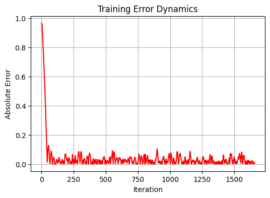
During the study, we conducted comprehensive testing of the system on historical data for the EURUSD currency pair. The time horizon was 5 years using the daily timeframe D1. Following conventional machine learning principles, we split the data into train and test sets in an 80/20 ratio. As a result, 1659 data points were used for training and 415 for testing. The model went through 20 training iterations with different weight initializations to find the optimal configuration.

Performance analysis

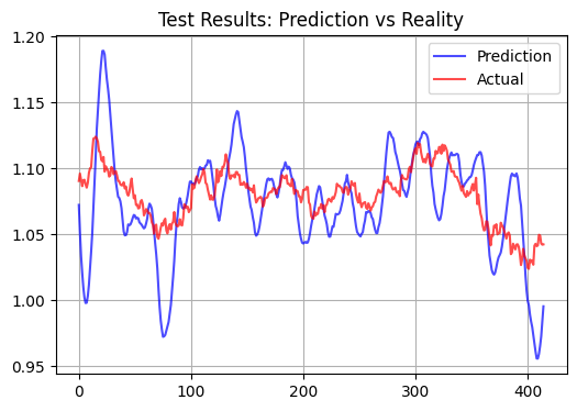
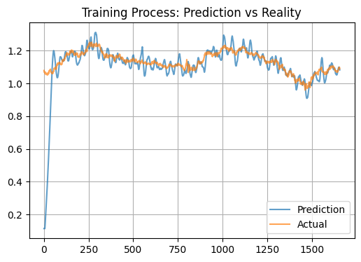
While analyzing the results, we discovered an interesting feature of our model. Instead of trying to predict short-term price movements, the system appears to aim to determine some kind of "fair" price for the currency pair. This observation is confirmed by the rather high correlation on the training sample, reaching the value of 0.583 with the relatively low standard error of 0.012346. However, on the test sample, the model's performance drops significantly: the correlation drops to negative values (-0.108), and the MSE increases more than 90 times, reaching 1.156584.

Comparison with traditional approaches

Our biologically inspired model exhibits significantly different behavior compared to classic technical indicators and standard neural networks. Its forecasts turn out to be significantly more volatile. 

Here is a test on a test sample, with a forecast horizon of 15 bars:

Statistical performance metrics

The most significant result of the model performance was the extremely low ratio of determination (R²) on the test sample, which amounted to approximately 0.01. Interestingly, the model shows a fairly high correlation on the training sample, which indicates its ability to capture long-term patterns in the data. Besides, the model forecasts often contain clearly visible spikes. Whether these spikes correspond to the smallest price movements and whether this is suitable for scalping remains to be seen.

Features and practical application

The observed behavior of the model can be explained by its biological nature. The plasma-like neural system appears to act as a powerful filter, significantly amplifying market signals, and the model produces exaggerated incremental forecasts. The STDP (Spike-Timing-Dependent Plasticity) mechanism, in theory, should lead to the formation of stable activation patterns, which leads to averaging of predictions, and, accordingly, we should get a different picture of the test and the actual state. An additional factor may be a large number of input in the form of technical indicators, which creates an overregularization effect.

From a practical point of view, this model can be used to determine short-term levels of fair value of a currency pair. 

Conclusion

Our research into a biologically inspired neural system for predicting financial markets has yielded unexpected but intriguing results. Just as the human brain is able to intuitively sense the "fair" value of an asset, our model, based on the working principles of living neurons, has demonstrated a remarkable ability to identify fundamentally sound price levels.

The introduction of a plasma-like environment into the neural network architecture created a kind of "collective intelligence," where each neuron influences the system's operation not only through direct connections, but also through long-range electromagnetic interactions. This mechanism has proven particularly efficient in sorting out market noise and identifying long-term trends. 

Perhaps there is a deeper meaning to this. Just as biological systems evolved to survive in the long term, our neural network, built in their image, also strives to identify stable, fundamentally sound patterns.

Bonus for those who read to the end

I also created an indicator based on this model. The indicator loads the rest of the system as a module and opens in a simple window like this:

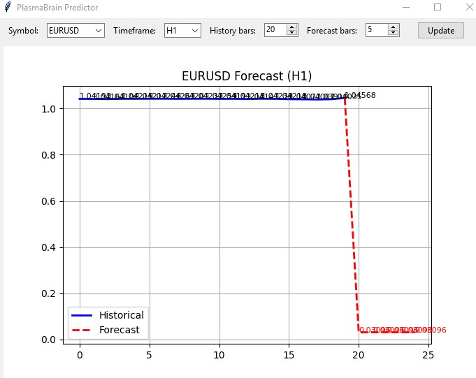
I have not tried it live, but considering that all the other systems generally predict the same direction, the indicator might work as it should.