Neural Networks in Trading: Training Deep Spiking Models (Conclusion)

Introduction

The financial market, like any complex nonlinear system, operates according to its own laws. It breathes, fluctuates, accumulates energy, and releases it in the form of sharp price movements. And the more closely we study its dynamics, the clearer it becomes that classical analytical methods can no longer always keep pace with the volatility of modern trading scenarios. A new generation of algorithms is taking their place — more sensitive, adaptive, and capable of seeing the market’s internal impulse beneath the surface of the chart.

In previous works, we have progressed from the basic principles of spiking computation to the implementation of key architectural solutions that pave the way for the practical use of such models in the MQL5 environment. Today, we are approaching the final stage of this journey — the implementation of the approaches proposed by the authors of the SEW ResNet (Spiking Elementary Weights Residual Network) framework, as applied to the analysis and forecasting of financial time series.

SEW ResNet owes its creation to the desire to combine the computational efficiency of spiking models with the robustness and depth of classic ResNet architectures. At the heart of this approach is the concept of energy-balanced learning, in which information is transmitted through a series of discrete pulses. Every spike carries weight-related meaning; every delay reflects the system's response to the signal. As a result, the model is not only more computationally efficient but also captures cause-and-effect relationships between events over time more accurately — which is particularly important for analyzing price impulses and bursts of market activity.

In the context of financial markets, this opens up new opportunities. After all, the market signal is spiking by nature. It is uneven, containing periods of silence and bursts of activity, where a single moment separates chaos from regularity. Under such conditions, classical neural networks often get stuck on noise or lose sensitivity during prolonged fluctuations. SEW ResNet, on the other hand, is designed to maintain responsiveness — it reacts only to truly significant changes in the data stream, naturally filtering out everything unnecessary.

In the previous stages, we built the foundation for the future architecture step by step. Each module we implemented became a building block in the framework's foundation, where technical rigor was combined with the intuitive logic of market processes.

The module for spiking activation with adaptive thresholds became the first key element of this system. Its function is to control the neuron's response to the incoming stream of signals by distinguishing important fluctuations from natural noise. In classical spiking models, activation is fixed and often responds identically to any change. We, on the other hand, took the approach of a biological prototype: the adaptive threshold changes depending on the intensity of the input pulses and the frequency of the spikes. As a result, the network learns to respond only when it is truly necessary, avoiding overfitting to random price fluctuations.

This has direct practical implications for the market. This mechanism allows the algorithm to operate reliably under conditions of high volatility, where traditional models often lose accuracy. When the chart is chaotic, the adaptive threshold acts as a built-in filter for market noise, helping the system maintain clarity and respond only to key trend changes.

The next step was the implementation of a gating mechanism responsible for regulating the neuron's sensitivity to the novelty of the incoming signal. Essentially, the gate determines how strongly the current signal should affect the buildup of membrane potential. In other words, it regulates the extent to which a new impulse contributes to the formation of the neuron's internal state. This gives the system dynamic flexibility. It is capable of responding differently to recurring and new patterns, gradually developing its own sense of habituation to similar events.

In financial market terms, this resembles the behavior of an experienced trader who does not react to every price movement but pays attention only to truly new signals that disrupt the established balance. The gating mechanism acts as a regulator of the model’s attentiveness — it determines when to amplify the response and when, conversely, to reduce it, thereby maintaining stable perception. This type of sensitivity control allows false signals to be filtered out without losing the ability to learn from actual changes in market dynamics.

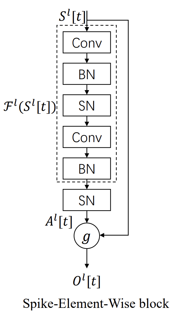
The implementation of the approaches proposed by the authors of the SEW ResNet framework in our work is based on the ResNeXt architecture, modified to accommodate spiking dynamics and adaptive sensitivity. At the heart of this approach is the concept of multi-channel perception, in which each parallel branch of the model processes data from its own perspective, and the results are then carefully combined into a single vector of market perception. This approach allows the model not only to register a price movement but also to distinguish its nature, intensity, and direction — things that traders typically determine by intuition.

The key component of the model is the Spike ResNeXt Bottleneck module, which acts as a kind of semantic filter. It compresses the incoming stream of signals, passes it through a narrow channel, and then expands it back out — but now in a cleaned, structured form. Here, the concept of the classic Bottleneck takes on a spiking dimension. Each element of the block is capable of deciding when to respond and when to remain silent.

The Bottleneck implementation uses a dynamic array of cBottleneck components that form the block's computational path. Layers are created programmatically, based on user-defined parameters. The data stream undergoes a series of sequential transformations: convolution operations, normalization, spiking activation, and grouped convolutions. The entire chain is designed to provide a balanced combination of accuracy and response speed.

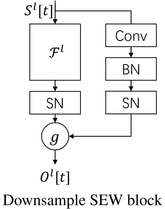
Equally important is the Spike ResNeXt Residual module, which is responsible for passing on accumulated experience. Its structure ensures correct dimensional alignment between the main path and the shortcut path, allowing information about previous states to be preserved without distortion. In a financial context, this is analogous to a trader's memory — the ability to recall what happened before the current impulse and adjust the response with history in mind.

The Residual block is implemented based on the same dynamic principle: if the input and output dimensions do not match, intermediate convolutional and normalization layers are added. This approach makes the architecture robust to changes in model parameters, allowing the network depth to be scaled freely without disrupting the internal logic of the signals.

A particular advantage of this approach is energy efficiency. The implemented zero-input check eliminates unnecessary computations when the market is silent. During periods of low volatility, many neurons simply do not fire, which reduces the load on the system and speeds up computations without sacrificing accuracy. This principle aligns with the natural economy of attention: the model focuses only on those areas of the market where something important is actually happening.

The combination of the multi-channel ResNeXt architecture and adaptive SEW spiking logic creates a unique hybrid in which mathematical precision meets market intuition. Each branch of the model is trained to form its own perspective on the data, and residual connections ensure that these perspectives are merged into a single solution. As a result, the model demonstrates robustness to noise and the ability to identify subtle patterns — the very faint signals that herald the emergence of a trend.

The practical value of this approach is clear: the model does not simply analyze the past, but learns to recognize moments when the market state changes. This provides an advantage in developing forecasting strategies, filtering out false signals, and automatically managing trading decisions.

The author’s visualization of the framework is shown below.

Key Principles of Implementation

After the individual modules had been implemented one by one, a natural question arose: how could we combine these elements into a single, cohesive architecture, where each part complements the others and the entire system functions as a unified whole?

However, we should not rush things here. The architecture should not merely connect blocks, but rather ensure harmonious interaction between processing levels, where low-level features seamlessly transition into more abstract market structures. Therefore, it makes sense to first examine the very foundation — the framework upon which our spiking intelligence will be built. As mentioned earlier, this framework was ResNeXt, known for its modular flexibility and high performance.

We took ResNeXt as the foundation, but gave it a spiking signal nature. In its classic form, ResNeXt analyzes data streams using parallel processing branches, each of which extracts a distinct aspect of the input data. In our implementation, these branches have been converted into spiking channels capable of independently adjusting their sensitivity and response frequency to market changes.

The Spike Bottleneck module already implements a basic sequence processing loop: the signal is compressed, transformed, and then expanded again, while preserving the semantic integrity of the data. This method works very well when analyzing univariate time series, where the relationship between the elements of the sequence is homogeneous. However, the market is more complex than that. We are dealing with a multimodal temporal structure in which interconnected processes — price, volume, volatility, liquidity, open interest, and many other features — unfold in parallel.

Attempting to analyze each of these channels independently, as a separate univariate sequence, results in the loss of critical information. There is a close, dynamic relationship among these features: changes in volume affect the amplitude of price fluctuations, volatility determines the market’s rhythm, and liquidity determines the depth of the market’s reaction to external influences. When these signals are processed separately, this interrelationship breaks down, and the model loses its ability to perceive the structural integrity of market behavior.

To address this shortcoming, in our implementation we introduce a second Bottleneck that operates on a transposed representation of the original tensor. Unlike standard analysis of univariate sequences, this block examines the data on a per-time-step basis, analyzing all channels simultaneously at each point in time. This allows the model to identify cross-channel relationships, track their dynamics, and account for the complex interactions between features.

At the same time, we retain only one Residual block to avoid unduly amplifying the influence of residual connections. This approach strikes a balance between preserving information about past states and efficiently processing new signal combinations. As a result, the model can simultaneously:

• extract local patterns within each univariate sequence;
• capture inter-channel dependencies and the coordinated dynamics of features;
• maintain robustness to noise and an excess of signals by limiting residual connections.

The hybrid approach transforms the SEW ResNeXt architecture into a tool capable of seeing the market as a complex dynamic system: each feature is interconnected with the others, and changes to a single element are reflected throughout the entire model structure.

The next important aspect to discuss is the choice of an element-wise spike-combination function for our three information streams. From the perspective of a risk-oriented approach and the binary nature of spikes, element-wise multiplication appears to be an attractive option. In this case, the signal is passed through only when it is confirmed across all streams simultaneously. This principle can be compared to a cautious trader who opens a position only when every indicator has confirmed the signal.

At first glance, the solution seems logical and rigorous — the model responds only to consistent information, thereby reducing the risk of false positives. However, it is worth taking a closer look at how the error gradient is distributed in this case.

If the signal is confirmed across all information streams, the error gradient is distributed evenly. However, if at least one stream has not generated a spike, the gradient is directed exclusively toward that stream, while the others receive zero correction. From a logical standpoint, this makes sense. When at least one stream returns zero, there is no downstream signal, and that particular stream requires correction. The error gradient signals that the given stream needs to be activated.

The problem arises in the critical case, when all information streams remain closed. In this scenario, each element of the element-wise multiplication is zero, and the error gradient, multiplied by these zeros, is completely blocked. As a result, the neuron stops receiving feedback — it is dead, and its parameters degrade. In practice, this can cause training to stop for part of the network or even the entire model, especially if such situations occur frequently.

In other words, strict element-wise multiplication becomes a trap for training. It protects against false signals, but at the same time creates the risk of neurons shutting down completely.

The unimpeded propagation of error gradients is ensured by simple summation of values, as implemented in the classic ResNet. This approach ensures that even if all information streams are temporarily blocked, the error gradient will be able to adjust the neuron's parameters, and training will continue without interruption.

However, this conflicts with the concept of spikes. Unlike a binary signal of “0” or “1,” the sum of several active streams can result in values of 2 or 3. This disrupts the spiking nature of the activation and can lead to undesirable oversignaling, where the model responds too sharply. In market terms, this is similar to a trader who opens a position with excessive confidence without any real data to back it up.

After weighing all the risks, we arrived at a more balanced design: we normalize the sum of the values of the information streams and then apply spiking activation. This allows us to simultaneously preserve the binary interpretation of the signal and ensure the correct propagation of error gradients. Normalization limits the resulting value to an acceptable range, preventing excessive responses, and also makes it possible to generate a reverse signal. This signal arises when multiple streams simultaneously block activation, and the network receives information indicating that reverse correction is necessary. Analogous to a cautious trader who reduces their position when faced with sharp opposition from market signals.

Top-Level Module

To implement the proposed concept in practice, we created a new object, CNeuronSpikeResNeXtBlock, which neatly integrates all the key elements of our architecture.

class CNeuronSpikeResNeXtBlock   :  public CNeuronSpikeActivation
  {
protected:
   CNeuronTransposeOCL           caTranspose[2];
   CNeuronSpikeResNeXtBottleneck caBottleneck[2];
   CNeuronSpikeResNeXtResidual   cResidual;
   CLayer                        cG;
   //---
   virtual bool      feedForward(CNeuronBaseOCL *NeuronOCL) override;
   virtual bool      updateInputWeights(CNeuronBaseOCL *NeuronOCL) override;
   virtual bool      calcInputGradients(CNeuronBaseOCL *NeuronOCL) override;

public:
                     CNeuronSpikeResNeXtBlock(void) {};
                    ~CNeuronSpikeResNeXtBlock(void) {};
   //---
   virtual bool      Init(uint numOutputs, uint myIndex, COpenCLMy *open_cl,
                          uint chanels_in, uint chanels_out, uint units_in,
                          uint units_out, uint group_size, uint groups,
                          ENUM_OPTIMIZATION optimization_type, uint batch);
   //---
   virtual int       Type(void)   override const   {  return defNeuronSpikeResNeXtBlock;   }
   //--- methods for working with files
   virtual bool      Save(int const file_handle) override;
   virtual bool      Load(int const file_handle) override;
   //---
   virtual void      SetOpenCL(COpenCLMy *obj) override;
   //---
   virtual bool      WeightsUpdate(CNeuronBaseOCL *source, float tau) override;
   virtual void      TrainMode(bool flag) override;
   virtual bool      Clear(void) override;
  };

It is based on two Bottleneck blocks, one Residual block, and transposed representations of the input data, which allows it to account for individual univariate sequences and complex cross-channel interactions. By extending CNeuronSpikeActivation, this class preserves the spiking nature of the signals and integrates gates with adaptive thresholds, enabling neurons to respond flexibly to changes in market dynamics.

One of the block's key elements is a dynamic array for storing pointers to cG spike-combination function objects, which significantly expands the block's capabilities and opens up room for experimentation. This array makes it possible to connect and use various methods of element-wise signal combination, including both simple summation and normalized combination followed by spiking activation. Thanks to this design, the block becomes not just a fixed structure, but a flexible platform for testing various signal integration strategies, adapting to the specific characteristics of particular market data.

The preparation of a new block is entirely handled by the Init method, which is responsible for initializing all of its key components and configuring how they interact.

bool CNeuronSpikeResNeXtBlock::Init(uint numOutputs, uint myIndex, COpenCLMy *open_cl,
                                    uint chanels_in, uint chanels_out, uint units_in,
                                    uint units_out, uint group_size, uint groups,
                                    ENUM_OPTIMIZATION optimization_type, uint batch)
  {
   if(!CNeuronSpikeActivation::Init(numOutputs, myIndex, open_cl, chanels_out * units_out,
                                    optimization_type, batch))
      return false;

Its algorithm begins by calling the method of the same name in the parent class, providing the foundation for spiking processing and the integration of gates with adaptive thresholds.

Next, the method initializes the transposed representations of the original tensor. The first object prepares the data for univariate sequence analysis, while the second performs the inverse transposition of the data. This approach allows the model to simultaneously account for the structure of individual information streams and the interactions between them, laying the foundation for the correct propagation of signals and gradients.

   uint index = 0;
   if(!caTranspose[0].Init(0, index, OpenCL, units_in, chanels_in, optimization, iBatch))
      return false;
   index++;
   if(!caTranspose[1].Init(0, index, OpenCL, chanels_out, units_out, optimization, iBatch))
      return false;

The next step is to initialize the Bottleneck blocks. The first Bottleneck processes classic univariate sequences, identifying local patterns in the signals, while the second works with a transposed representation, capturing inter-channel dependencies and the coordinated dynamics of features. Each block receives the channel parameters, the number of groups, and the group size, as well as the necessary optimization parameters and batch size.

   index++;
   if(!caBottleneck[0].Init(0, index, OpenCL, chanels_in, chanels_out, units_in, units_out,
                            group_size, groups, optimization, iBatch))
      return false;
   index++;
   if(!caBottleneck[1].Init(0, index, OpenCL, units_in, units_out, chanels_in, chanels_out,
                            group_size, groups, optimization, iBatch))
      return false;

The method then initializes the Residual block, which preserves critical residual connections, ensuring stability and a balance between a neuron's memory and adaptability.

   index++;
   if(!cResidual.Init(0, index, OpenCL, chanels_in, chanels_out, units_in, units_out,
                      optimization, iBatch))
      return false;

Finally, the method creates cG, which contains a dynamic array of spike-combination function objects. Here, a base neuron without activation and a batch normalization object are added sequentially. This sequence allows signals from different information streams to be correctly summed and normalized.

   CNeuronBaseOCL*      neuron = NULL;
   CNeuronBatchNormOCL* norm = NULL;
   cG.Clear();
   cG.SetOpenCL(OpenCL);
   index++;
   neuron = new CNeuronBaseOCL();
   if(!neuron ||
      !neuron.Init(0, index, OpenCL, Neurons(), optimization, iBatch) ||
      !cG.Add(neuron))
     {
      DeleteObj(neuron)
      return false;
     }
   neuron.SetActivationFunction(None);
//---
   if(!cResidual.SetGradient(neuron.getGradient(), true) ||
      !caTranspose[1].SetGradient(neuron.getGradient(), true) ||
      !caBottleneck[0].SetGradient(neuron.getGradient(), true))
      return false;
//---
   index++;
   norm = new CNeuronBatchNormOCL();
   if(!norm ||
      !norm.Init(0, index, OpenCL, Neurons(), iBatch, optimization) ||
      !cG.Add(norm))
     {
      DeleteObj(norm)
      return false;
     }
//---
   return true;
  }

In addition, the block provides synchronization of pointers to error gradient buffers for key components, which ensures correct error propagation throughout the network without unnecessary data copying and prevents signal degradation.

As a result, the Init method creates a fully ready block in which every component is initialized, configured, and connected to the others.

The forward pass of the signals is implemented in the feedForward method, which ensures sequential processing of information through all key components of the SEW ResNeXt block.

bool CNeuronSpikeResNeXtBlock::feedForward(CNeuronBaseOCL *NeuronOCL)
  {
   if(!caTranspose[0].FeedForward(NeuronOCL))
      return false;

First, the data passes through the first transposed block, creating a representation of time steps for further analysis. The signal is then processed sequentially by the first Bottleneck module, which identifies local patterns in univariate sequences.

   if(!caBottleneck[0].FeedForward(NeuronOCL))
      return false;

The second Bottleneck, in turn, operates on the output of the transposed block, capturing inter-channel dependencies and the coordinated dynamics of features.

   if(!caBottleneck[1].FeedForward(caTranspose[0].AsObject()))
      return false;
   if(!caTranspose[1].FeedForward(caBottleneck[1].AsObject()))
      return false;

The information then passes through a second transposed block, preparing it for integration with the residual connections provided by the Residual block*.

   if(!cResidual.FeedForward(NeuronOCL))
      return false;

The next step involves combining the spikes. Signals from both the Bottleneck and Residual blocks are summed.

   CNeuronBaseOCL* current = cG[0];
   if(!current)
      return false;
   if(!SumAndNormilize(caBottleneck[0].getOutput(), caTranspose[1].getOutput(),
                       current.getOutput(), caTranspose[1].GetCount(), false, 0, 0, 0, 1) ||
      !SumAndNormilize(current.getOutput(), cResidual.getOutput(),
                       current.getOutput(), caTranspose[1].GetCount(), false, 0, 0, 0, 1))
      return false;

This approach allows both univariate and inter-channel signals to be correctly integrated, preserving the binary nature of spikes and preventing neuron degradation.

Next, the remaining elements of the cG array undergo their own forward pass, where each object receives the output of the previous neuron as its input, ensuring the sequential propagation of signals through all combination functions.

   for(int i = 1; i < cG.Total(); i++)
     {
      current = cG[i];
      if(!current ||
         !current.FeedForward(cG[i - 1]))
         return false;
     }
//---
   return CNeuronSpikeActivation::feedforward(cG[-1]);
  }

The process concludes by calling the method of the same name in the parent class, which performs the final processing of the spiking signals and passes the results to the next level of the model.

Thus, the forward pass algorithm ensures smooth, structured signal propagation through all components of the block, integrating local and inter-channel dependencies, normalizing the combined spikes, and preserving correct propagation of error gradients for training. In a market context, this allows the model to respond simultaneously to local changes in each data stream and to the coordinated dynamics of the features, creating a stable and adaptive system for analyzing financial data.

Correct gradient distribution is implemented in the calcInputGradients method, which ensures consistent and coordinated updating of the parameters of all components in the SEW ResNeXt block.

bool CNeuronSpikeResNeXtBlock::calcInputGradients(CNeuronBaseOCL *NeuronOCL)
  {
   if(!NeuronOCL)
      return false;

The method begins by verifying the validity of the pointer to the source data object and calling the method of the same name in the parent class, which ensures that gradients are propagated correctly up to the last layer of the cG spike combination module.

   if(!CNeuronSpikeActivation::calcInputGradients(cG[-1]))
      return false;

Next, we iterate through all elements of the dynamic cG array in reverse order, from last to first, computing the hidden gradients of each neuron based on the output of the next neuron in the chain.

   CNeuronBaseOCL* current = NULL;
   for(int i = cG.Total() - 2; i >= 0; i--)
     {
      current = cG[i];
      if(!current ||
         !current.CalcHiddenGradients(cG[i + 1]))
         return false;
     }

This approach allows the error to be correctly distributed across all combination and normalization functions, ensuring consistent learning at the spike level.

It should be noted here that, because the pointers to the error-gradient buffers of the main components are swapped, once the error is propagated to the first element of the cG array, it is automatically propagated to all information streams within the block. This technique ensures that each stream receives the correct feedback without the need to manually synchronize the gradients for each component. As a result, error propagation occurs naturally and continuously, ensuring consistent training across the entire block structure and preventing neuron degradation even in the presence of complex, interdependent signals.

The resulting gradients are then passed to the second Bottleneck and the transposed block, capturing the effect of inter-channel dependencies on the model's error.

   if(!caBottleneck[1].CalcHiddenGradients(caTranspose[1].AsObject()))
      return false;
   if(!caTranspose[0].CalcHiddenGradients(caBottleneck[1].AsObject()))
      return false;

The backpropagated error is then propagated through the Residual block, which allows the residual connections to be adjusted without unduly amplifying the influence of previous signals.

   if(!NeuronOCL.CalcHiddenGradients(cResidual.AsObject()))
      return false;

Special attention has been paid to ensuring the accurate storage of data from all information streams. To do this, a temporary data buffer is used, which collects information about the error and correctly feeds it back to the inputs. This prevents the formation of dead neurons, ensuring stable and continuous learning even when signals are temporarily absent in individual streams.

   CBufferFloat* temp = NeuronOCL.getGradient();
   if(!NeuronOCL.SetGradient(caTranspose[0].getPrevOutput(), false))
      return false;
   if(!NeuronOCL.CalcHiddenGradients(caBottleneck[0].AsObject()))
      return false;
   if(!SumAndNormilize(temp, NeuronOCL.getGradient(), temp,
                       caTranspose[0].GetWindow(), false, 0, 0, 0, 1))
      return false;
   if(!NeuronOCL.CalcHiddenGradients(caTranspose[0].AsObject()))
      return false;
   if(!SumAndNormilize(temp, NeuronOCL.getGradient(), temp,
                       caTranspose[0].GetWindow(), false, 0, 0, 0, 1))
      return false;
   if(!NeuronOCL.SetGradient(temp, false))
      return false;
//---
   return true;
  }

As a result, the calcInputGradients method ensures consistent and safe distribution of error gradients across all components of the block, from transposed sequences and Bottleneck modules to Residual and the spike combination block. This mechanism ensures that each neuron receives sufficient feedback, adjusts its parameters, and maintains the adaptability of the model, which is capable of analyzing complex multimodal market sequences.

The complete source code for the CNeuronSpikeResNeXtBlock class, including all implemented methods, is provided in the attachment, allowing you to study the block’s internal workings in detail and trace the signal processing logic at each stage.

Model Architecture

The next step in our work is to design the architecture of the trainable models. As before, we continue to work within the Actor-Critic framework, developing a model capable of making trading decisions independently and responding to market changes. We integrate all previously implemented SEW ResNeXt approaches into the Environment State Encoder, which acts as the model’s sensory organ, accumulating and processing all incoming market information.

bool CreateDescriptions(CArrayObj *&encoder,
                        CArrayObj *&actor,
                        CArrayObj *&critic
                       )
  {
//---
   CLayerDescription *descr;
//---
   if(!encoder)
     {
      encoder = new CArrayObj();
      if(!encoder)
         return false;
     }
   if(!actor)
     {
      actor = new CArrayObj();
      if(!actor)
         return false;
     }
   if(!critic)
     {
      critic = new CArrayObj();
      if(!critic)
         return false;
     }

The process of building the Encoder begins with initializing the layer array itself, after which an input layer is formed to receive raw data for price history and bar features.

//--- Encoder
   encoder.Clear();
//--- Input layer
   if(!(descr = new CLayerDescription()))
      return false;
   descr.type = defNeuronBaseOCL;
   uint prev_count = descr.count = (HistoryBars * BarDescr);
   descr.activation = None;
   descr.optimization = ADAM;
   if(!encoder.Add(descr))
     {
      delete descr;
      return false;
     }
   iLatentLayer = 0;

This is followed by a batch normalization layer with added noise, which ensures stability and smoothness during training.

//--- layer 1
   if(!(descr = new CLayerDescription()))
      return false;
   descr.type = defNeuronBatchNormWithNoise;
   descr.count = prev_count;
   descr.batch = BatchSize;
   descr.activation = None;
   descr.optimization = ADAM;
   if(!encoder.Add(descr))
     {
      delete descr;
      return false;
     }
   iLatentLayer++;

Then comes a ConcatDiff layer, which aggregates temporal differences to create the initial hidden representation.

//--- layer 2
   if(!(descr = new CLayerDescription()))
      return false;
   descr.type = defNeuronConcatDiff;
   prev_count = descr.count = HistoryBars;
   descr.layers = BarDescr;
   descr.step = 1;
   descr.batch = BatchSize;
   descr.optimization = ADAM;
   descr.activation = None;
   if(!encoder.Add(descr))
     {
      delete descr;
      return false;
     }
   iLatentLayer++;
   uint prev_out = descr.layers * 2 ;

Next, the Mamba4CastEmbedding layer is used, which encodes information about time intervals, preparing the data for more complex processing.

//--- layer 3
   if(!(descr = new CLayerDescription()))
      return false;
   descr.type = defMamba4CastEmbeding;
   prev_count = descr.count = HistoryBars;
   descr.window = prev_out;
   prev_out = descr.window_out = NSkills;
     {
      uint temp[] = {PeriodSeconds(PERIOD_D1), PeriodSeconds(PERIOD_MN1)};
      if(ArrayCopy(descr.windows, temp) < (int)temp.Size())
         return false;
     }
   descr.batch = BatchSize;
   descr.optimization = ADAM;
   descr.activation = None;
   if(!encoder.Add(descr))
     {
      delete descr;
      return false;
     }
   iLatentLayer++;

At the next stage, the NeuronSpikeResNeXtBlock layers are brought into operation; they are repeated multiple times and form a deep, multi-channel representation of the market state.

//--- layer 4
   if(!(descr = new CLayerDescription()))
      return false;
   descr.type = defNeuronSpikeResNeXtBlock;
     {
      uint temp[] = {prev_out,            // Channels In
                     prev_out,            // Channels Out
                     EmbeddingSize/2      // Group Size
                    };
      if(ArrayCopy(descr.windows, temp) < (int)temp.Size())
         return false;
     }
     {
      uint temp[] = {prev_count,          // Units In
                     prev_count,          // Units Out
                     NScenarios           // Number of Groups
                    };
      if(ArrayCopy(descr.units, temp) < (int)temp.Size())
         return false;
     }
   descr.optimization = ADAM;
   descr.batch = BatchSize;
   descr.activation = None;
   for(int i = 0; i < 2; i++)
      if(!encoder.Add(descr))
        {
         delete descr;
         return false;
        }
      else
         iLatentLayer++;
//--- Layer 5
   if(!(descr = new CLayerDescription()))
      return false;
   descr.type = defNeuronSpikeResNeXtBlock;
     {
      uint temp[] = {prev_out,              // Channels In
                     prev_out * 2,          // Channels Out
                     EmbeddingSize/2        // Group Size
                    };
      if(ArrayCopy(descr.windows, temp) < (int)temp.Size())
         return false;
     }
     {
      uint temp[] = {prev_count,            // Units In
                     prev_count / 2,        // Units Out
                     NScenarios             // Number of Groups
                    };
      if(ArrayCopy(descr.units, temp) < (int)temp.Size())
         return false;
     }
   descr.optimization = ADAM;
   descr.batch = BatchSize;
   descr.activation = None;
   if(!encoder.Add(descr))
     {
      delete descr;
      return false;
     }
   iLatentLayer++;
   prev_count = descr.units[1];
   prev_out = descr.windows[1];
//--- Layer 6
   if(!(descr = new CLayerDescription()))
      return false;
   descr.type = defNeuronSpikeResNeXtBlock;
     {
      uint temp[] = {prev_out,            // Channels In
                     prev_out,            // Channels Out
                     EmbeddingSize/2      // Group Size
                    };
      if(ArrayCopy(descr.windows, temp) < (int)temp.Size())
         return false;
     }
     {
      uint temp[] = {prev_count,          // Units In
                     prev_count,          // Units Out
                     NScenarios           // Number of Groups
                    };
      if(ArrayCopy(descr.units, temp) < (int)temp.Size())
         return false;
     }
   descr.optimization = ADAM;
   descr.batch = BatchSize;
   descr.activation = None;
   for(int i = 0; i < 2; i++)
      if(!encoder.Add(descr))
        {
         delete descr;
         return false;
        }
      else
         iLatentLayer++;
//--- Layer 7
   if(!(descr = new CLayerDescription()))
      return false;
   descr.type = defNeuronSpikeResNeXtBlock;
     {
      uint temp[] = {prev_out,              // Channels In
                     prev_out * 2,          // Channels Out
                     EmbeddingSize/2        // Group Size
                    };
      if(ArrayCopy(descr.windows, temp) < (int)temp.Size())
         return false;
     }
     {
      uint temp[] = {prev_count,            // Units In
                     prev_count / 2,        // Units Out
                     NScenarios             // Number of Groups
                    };
      if(ArrayCopy(descr.units, temp) < (int)temp.Size())
         return false;
     }
   descr.optimization = ADAM;
   descr.batch = BatchSize;
   descr.activation = None;
   if(!encoder.Add(descr))
     {
      delete descr;
      return false;
     }
   iLatentLayer++;
   prev_count = descr.units[1];
   prev_out = descr.windows[1];
//--- Layer 8
   if(!(descr = new CLayerDescription()))
      return false;
   descr.type = defNeuronSpikeResNeXtBlock;
     {
      uint temp[] = {prev_out,            // Channels In
                     prev_out,            // Channels Out
                     EmbeddingSize/2      // Group Size
                    };
      if(ArrayCopy(descr.windows, temp) < (int)temp.Size())
         return false;
     }
     {
      uint temp[] = {prev_count,          // Units In
                     prev_count,          // Units Out
                     NScenarios           // Number of Groups
                    };
      if(ArrayCopy(descr.units, temp) < (int)temp.Size())
         return false;
     }
   descr.optimization = ADAM;
   descr.batch = BatchSize;
   descr.activation = None;
   for(int i = 0; i < 2; i++)
      if(!encoder.Add(descr))
        {
         delete descr;
         return false;
        }
      else
         iLatentLayer++;
//--- Layer 9
   if(!(descr = new CLayerDescription()))
      return false;
   descr.type = defNeuronSpikeResNeXtBlock;
     {
      uint temp[] = {prev_out,            // Channels In
                     prev_out * 2,        // Channels Out
                     EmbeddingSize/2      // Group Size
                    };
      if(ArrayCopy(descr.windows, temp) < (int)temp.Size())
         return false;
     }
     {
      uint temp[] = {prev_count,          // Units In
                     prev_count / 2,      // Units Out
                     NScenarios           // Number of Groups
                    };
      if(ArrayCopy(descr.units, temp) < (int)temp.Size())
         return false;
     }
   descr.optimization = ADAM;
   descr.batch = BatchSize;
   descr.activation = None;
   if(!encoder.Add(descr))
     {
      delete descr;
      return false;
     }
   iLatentLayer++;
   prev_count = descr.units[1];
   prev_out = descr.windows[1];
//--- Layer 10
   if(!(descr = new CLayerDescription()))
      return false;
   descr.type = defNeuronSpikeResNeXtBlock;
     {
      uint temp[] = {prev_out,            // Channels In
                     prev_out,            // Channels Out
                     EmbeddingSize/2      // Group Size
                    };
      if(ArrayCopy(descr.windows, temp) < (int)temp.Size())
         return false;
     }
     {
      uint temp[] = {prev_count,          // Units In
                     prev_count,          // Units Out
                     NScenarios           // Number of Groups
                    };
      if(ArrayCopy(descr.units, temp) < (int)temp.Size())
         return false;
     }
   descr.optimization = ADAM;
   descr.batch = BatchSize;
   descr.activation = None;
   for(int i = 0; i < 2; i++)
      if(!encoder.Add(descr))
        {
         delete descr;
         return false;
        }
      else
         iLatentLayer++;
   uint window = prev_out;
   uint count = prev_count;

Each block receives the outputs of the previous block as its input, accounts for cross-channel dependencies, and normalizes the summed spikes, ensuring that signals are transmitted correctly throughout the entire network. Channel parameters, the number of groups, batch size, and optimization settings are selected so that the blocks can efficiently encode multimodal sequences and maintain adaptability even during sharp market fluctuations.

After a series of spiking blocks, the Encoder ends with convolution and transposition layers that consolidate the output representation and form the final hidden state vector intended to build a forecast of the upcoming movement in the analyzed market features. This tensor accumulates information about temporal and cross-channel dependencies, providing an accurate and consistent representation of the market state.

//--- Layer 11
   if(!(descr = new CLayerDescription()))
      return false;
   descr.type = defNeuronConvOCL;
   descr.count = prev_count;
   descr.window = prev_out;
   descr.step = prev_out;
   prev_out = descr.window_out = BarDescr;
   descr.activation = TANH;
   descr.optimization = ADAM;
   if(!encoder.Add(descr))
     {
      delete descr;
      return false;
     }
//--- Layer 12
   if(!(descr = new CLayerDescription()))
      return false;
   descr.type = defNeuronTransposeOCL;
   descr.count = prev_count;
   prev_count = descr.window = prev_out;
   descr.batch = BatchSize;
   descr.optimization = ADAM;
   descr.activation = None;
   if(!encoder.Add(descr))
     {
      delete descr;
      return false;
     }
   prev_out = descr.count;
//--- Layer 13
   if(!(descr = new CLayerDescription()))
      return false;
   descr.type = defNeuronConvOCL;
   descr.count = prev_count;
   descr.window = prev_out;
   descr.step = prev_out;
   prev_out = descr.window_out = NForecast;
   descr.activation = TANH;
   descr.optimization = ADAM;
   if(!encoder.Add(descr))
     {
      delete descr;
      return false;
     }
//--- Layer 14
   if(!(descr = new CLayerDescription()))
      return false;
   descr.type = defNeuronTransposeOCL;
   descr.count = prev_count;
   prev_count = descr.window = prev_out;
   descr.batch = BatchSize;
   descr.optimization = ADAM;
   descr.activation = None;
   if(!encoder.Add(descr))
     {
      delete descr;
      return false;
     }
   prev_out = descr.count;

The final layer, NeuronRevInDenormOCL, ensures that signals are correctly scaled and denormalized.

//--- layer 15
   if(!(descr = new CLayerDescription()))
      return false;
   descr.type = defNeuronRevInDenormOCL;
   descr.count = prev_count * prev_out;
   descr.layers = 1;
   if(!encoder.Add(descr))
     {
      delete descr;
      return false;
     }

The Actor and Critic architectures have been ported entirely from previous works without any changes, preserving their time-tested structure and functionality. You can find them in the attachment to this article. Thanks to this organization, our model receives a powerful Encoder capable of capturing complex temporal and cross-channel market dependencies, while the Actor and Critic use this representation for accurate forecasting and trading decisions.

Testing

We have completed a major effort to integrate the key components of the SEW ResNeXt framework, and now it is time to evaluate the effectiveness of the solutions we have implemented. Before entrusting the model with real funds, it is necessary to thoroughly test the strategy using historical and simulated data, as if honing the skills of an experienced trader and verifying its ability to perform under a wide variety of market conditions. Each stage simulates a live market, allowing the model to gradually gain experience, learn to distinguish signals from noise, and develop robust behavioral algorithms necessary for operating in a real trading environment.

The first stage — offline training — is based on historical data for the EURUSD currency pair on the H1 timeframe for the period from January 2024 through June 2025. This period served as a real training ground. The model was trained to reproduce historical patterns, understand price dynamics and trading volumes, and identify regularities and dependencies among key features. It could be said that the model developed a trader's intuition combined with precise strategic judgment. It gradually developed the ability to anticipate market movements and assess the risk of each potential trade.

The next stage — online fine-tuning in the MetaTrader 5 Strategy Tester — will allow the model to work with real-time data streams, candle by candle. Here, it masters the dynamics of the real market, learns to remain stable amid market noise, adjust its actions under low liquidity, and react instantly to sharp price spikes. This stage served as a sort of final refinement of the strategy. The basic structure, built on historical data, remained unchanged, but the model learned to respond flexibly to current market conditions, minimizing the risk of overfitting and improving the accuracy of forecasts even in a volatile environment.

The final test was conducted using data from July–September 2025 — data that was entirely new and had not been used before. All parameters obtained in the previous stages were loaded without modification, which ensured a fair assessment of the model's ability to generalize. Test results confirm that a step-by-step approach to training and adaptation enables the model to analyze the market and generate a forecast of the upcoming movement of key market features, which can be relied upon when making real trading decisions.

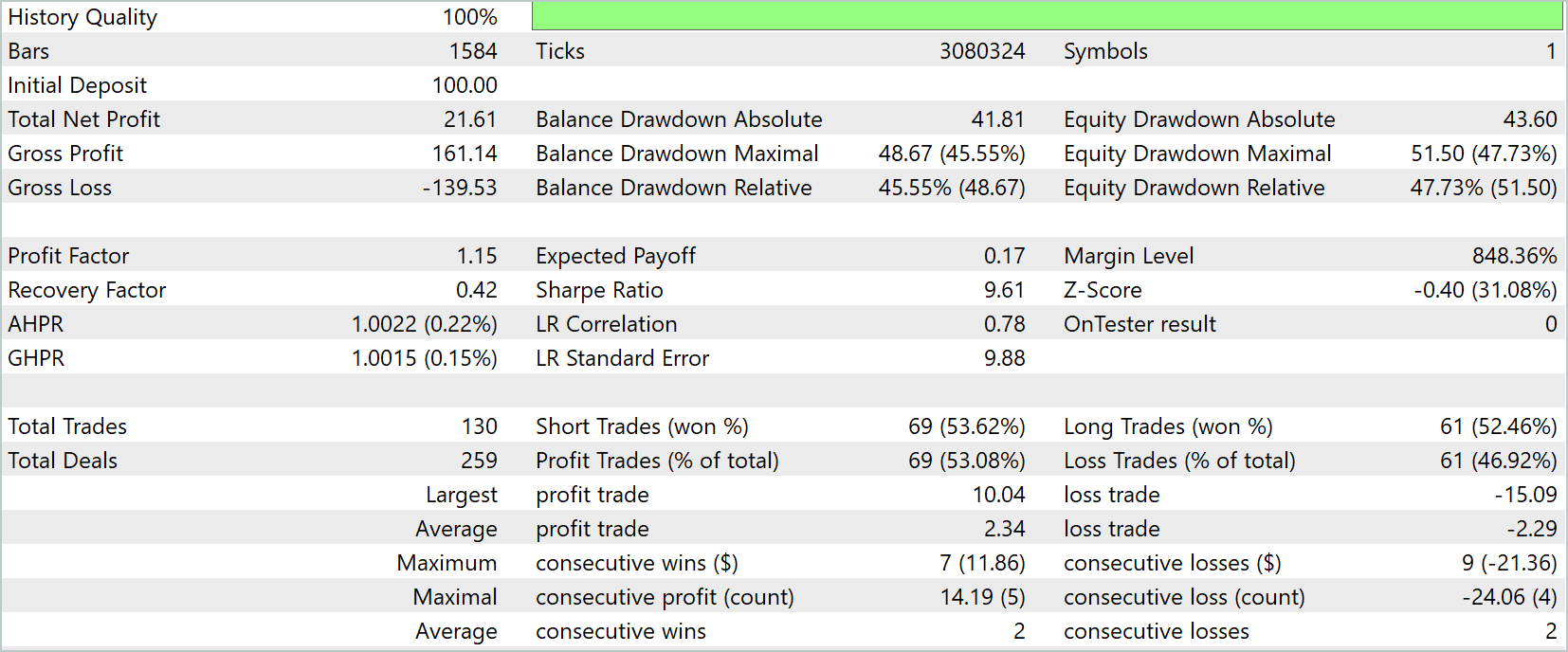
The balance and equity chart shows steady capital growth throughout virtually the entire testing period. Despite occasional drawdowns, equity remains close to the balance. This indicates a prudent and controlled risk management strategy. The maximum equity drawdown was 47.73%, which is quite high under volatile conditions but is consistent with the test scenarios for a time period characterized by sharp price fluctuations.

Total profit amounted to 21.61 USD on an initial deposit of 100.0 USD, representing capital growth of more than 20% over the period under review. The Profit Factor is 1.15. This indicates that total profits exceed total losses, and the Sharpe ratio of 9.61 demonstrates the strategy’s high risk-adjusted performance. The Recovery Factor is 0.42. It reflects the need to focus on drawdown management when extrapolating to larger amounts of capital.

The model executed 130 trades, of which slightly more than half were profitable (53.08%), and the average profit per trade was 2.34 USD, while the average loss was 2.29 USD. The longest winning streak was 7 trades, with a total profit of 11.86 USD, while the longest losing streak was 9 trades, with a total loss of 21.36 USD. These metrics demonstrate the strategy's moderate aggressiveness and the model's ability to adapt to short-term market fluctuations.

It is worth paying special attention to the even distribution of trades between short and long positions: 69 short trades and 61 long trades, with success rates of 53.62% and 52.46%, respectively. This indicates that the model behaves in a balanced manner across various market scenarios and is capable of responding to both rising and falling prices.

Overall, the test results confirm the viability of the constructed framework based on SEW ResNeXt with elements of spiking activation. The model demonstrates stability, adaptability to market dynamics, and sound risk management, making it suitable for further work under real-world financial market conditions.

Conclusion

We have completed the practical implementation of the approaches proposed by the authors of the SEW ResNet framework and built a working platform in which every detail serves a practical purpose. Spiking activations with adaptive thresholds taught the model to respond with restraint. Gates added sensitivity to novelty. The two Bottleneck blocks provided a compromise between local analysis and accounting for cross-channel dependencies. The residual block preserved memory but did not let it stifle adaptation.

The test results confirmed that the concept works. Capital growth of 21.6% is an objective indicator of performance. A Profit Factor of 1.15 and a win rate of just over 50% indicate that the signal logic is viable. The average profit and the average loss are similar in magnitude — the model does not rely on rare, lucky trades. That said, a maximum drawdown of 47% is a serious challenge that cannot be ignored.

The strengths of the implementation are obvious. The model effectively filters out market noise. It sees interrelationships between channels that are lost when they are analyzed separately. The architecture preserves gradient flow and remains trainable even in challenging scenarios. The code is modular. OpenCL integration paves the way for acceleration and scalability.

At the same time, there are also areas that need further work. A high maximum drawdown requires enhanced risk management. Tests in a simulator are not the same as real trading: expected slippage, spreads, and market liquidity can alter profit and loss profiles. The sample size and the specific time period also play a role — thorough validation is needed using new data and across different market conditions.

The practical conclusion is simple: the architecture has proven itself as a platform for research and practical application. It provides the trader with a tool that can be debugged, interpreted, and improved. But that's not the end of the road.

Links

• Deep Residual Learning in Spiking Neural Networks
• Other articles in this series

Software used in the article

#	Name	Type	Description
1	Study.mq5	Expert Advisor	Expert Advisor for offline model training
2	StudyOnline.mq5	Expert Advisor	Expert Advisor for online model training
3	Test.mq5	Expert Advisor	Expert Advisor for model testing
4	Trajectory.mqh	Class Library	Structure describing the system state and model architecture
5	NeuroNet.mqh	Class Library	Class library for building a neural network
6	NeuroNet.cl	Library	Code library for an OpenCL program