Neural Networks in Trading: Training Deep Spiking Models (Spike Integration)

Introduction

Financial markets have always been a battleground of opposing forces: order and chaos, rational calculation and irrational emotional outbursts. They resemble a stormy sea, where the surface reveals the play of waves — price fluctuations — while complex currents lie hidden beneath the water: fundamental factors, macroeconomic shifts, and the psychological sentiment of market participants. In this world, every trader, investor, or researcher is searching for the key to understanding patterns. Some rely on intuition, others on rigorous formulas, but in recent decades more and more attention has been focused on artificial intelligence and neural network architectures.

Classical neural networks, designed for processing images and audio, seemed to be universal tools. But when we apply them to the field of financial time series — especially high-frequency data — fundamental contradictions come to light. The market is not the smooth curve of a function, but a stream of events: trades, orders, spikes in volatility, and surges in liquidity. It is a series of discrete metronome beats, where each price tick can be viewed as a pulse. That is precisely why spiking neural networks (SNN, Spiking Neural Networks) have attracted the attention of researchers in recent years. They are closer to the very nature of the market, where everything is measured by a sequence of events over time.

But the shift from classical models to spiking models is not just a technical detail — it is a fundamental paradigm shift. What works in a world of smooth activations may prove useless in a spiking context. A prime example is the well-known ResNet architecture. In its classical form, ResNet revolutionized machine learning by making it possible to build networks with dozens or even hundreds of layers without sacrificing trainability. The secret lay in shortcut connections, which allowed the signal and the gradient to pass through the network with almost no distortion.

And this is important to emphasize. In a standard model, a ResNet shortcut is not a pure layer bypass. It, too, is passed through the ReLU activation function. However, since ReLU is positive and continuous, the shortcut is propagated almost identically, and gradients flow freely. It is precisely this characteristic that has made ResNet a symbol of depth and stability.

The situation is quite different with spiking models. Here, activation is a binary pulse. When a shortcut is subjected to a spiking activation function, it loses its identity. Binarization undermines the very concept of a shortcut as a direct channel. As a result, depth ceases to function: gradients either vanish or become unstable, and the network loses its ability to learn. Here, the authors of SEW-ResNet proposed a solution that can be described as both simple and ingenious.

They moved the shortcut outside the scope of the activation function. Instead of passing it through binary activation, they kept the shortcut separate and combined it with the result of the residual transformation after activation, defining this combination as a separate element-wise operation. In this way, the shortcut regains its true purpose. It is truly an identity path, and the signal is not lost in the discrete dynamics.

This change may seem minor, but its implications are enormous. Now, deep spiking models are once again trainable. This means we can build models with dozens of layers and expect them to perform just as stably as their predecessors in the world of classical neural networks.

In addition, the authors of SEW-ResNet expanded the concept of the shortcut. In the classic ResNet, the combination operation was fixed: simple addition. In SEW-ResNet, there is room for choice: addition, logical AND, its inversion, and other functions g(•,•). This opens a new chapter in architecture design. The shortcut can be tailored to a specific task.

In a financial context, this is particularly valuable. Imagine the foreign exchange market. Short impulses triggered by news events are superimposed on long-term trends shaped by central bank policy. Stocks are characterized by seasonal fluctuations and the impact of quarterly earnings reports, while cryptocurrencies see sudden surges in community activity and technological updates. A single architecture isn't enough for all processes — flexibility is needed. SEW-ResNet provides it. You can choose a shortcut that better captures the unique characteristics of a specific asset.

For traders and researchers, this means a new level of analysis. While traditional methods can capture only the market’s average state, SEW-ResNet makes it possible to simultaneously sense rapid market ticks and long-term movements. The shortcut becomes something like a reliable memory channel that prevents the model from forgetting what happened earlier, while still allowing it to perceive new events.

SEW-ResNet can be viewed as an important step in the evolution of spiking models. This is a fundamental restoration of the key depth mechanism under binary dynamics.

The authors’ visualization of the framework is shown below.

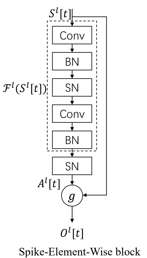
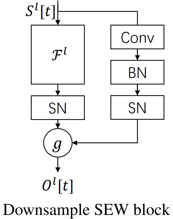
In the practical section of the previous article, we focused on the fundamental elements of a spiking neuron adapted for financial time series. Particular attention was paid to two key mechanisms:

• trainable activation thresholds;
• membrane potential accumulation gates.

A trainable activation threshold will allow the neuron to flexibly adjust its sensitivity to input pulses. In market terminology, this is similar to adjusting for volatility. The neuron learns to distinguish between random price fluctuations and truly significant events. As a result, even in a highly volatile market, the model retains the ability to respond only to significant signals, avoiding an excess of false spikes.

Membrane potential accumulation gates control the integration of the events being analyzed. Instead of simply summing incoming spikes, the neuron controls the accumulation of potential and determines when it leads to the generation of a spike. This feature will allow the model to build temporal memory — to record sequences of significant events and decide to generate a spike only when the accumulated signal exceeds a threshold adapted to the current market context.

These mechanisms were implemented at the level of the basic spiking neuron, creating a platform for building more complex architectures.

Optimizing an OpenCL Program

Today, we are continuing the work we started. But before we move on to implementing the approaches proposed by the authors of the SEW-ResNet framework, let’s take a brief detour and consider another important feature of spiking models — the neuron remaining silent until an event occurs. This property significantly reduces computational costs, since the neuron waits for a signal and does not expend resources processing empty inputs. In the algorithms we have implemented previously, a zero input does not result in any resource savings. The operation of multiplying by zero was performed every time, even though the result was known in advance.

In classical neural network models, this behavior is entirely justified. A zero input is rare — an exception to the rule — and introducing additional checks often only complicates and slows down computation. But spiking models work differently. Here, most inputs are zero at any given moment, since only isolated events — short pulses against a background of silence — are significant. Therefore, adding a zero-value check that allows operations involving zeros to be skipped becomes a natural and justified solution.

If we draw a parallel with financial markets, a neuron’s silence resembles the “quiet” on a chart between spikes in trading activity. During periods when the market is calm, each price tick provides little information — and analyzing each one would be a waste of resources. A spiking neuron behaves in a similar way. It remains inactive until it receives a signal carrying meaningful information. As soon as an event occurs (a sharp spike in volume, a breakout, or a news-driven impulse), the neuron reacts instantly. This approach conserves computational resources and improves the network's resilience to noise by filtering out insignificant changes that have no value.

However, in order to preserve the versatility of our library's components, we chose not to create new objects but instead decided to add zero-value checks to the existing algorithms. Let's start with the forward pass of the fully connected layer, where the most significant changes were made to the kernel of the OpenCL program.

First, a zero-value check was added for the data being analyzed. Second, we abandoned the classic loop over all input data within a single work-item. Instead, the computations are distributed among the work-items in the work-group, and the results are summed after all work-items have finished. This approach significantly improves efficiency and makes it possible to use the parallel processing capabilities of the GPU.

__kernel void FeedForward(__global const float *matrix_w,
                          __global const float *matrix_i,
                          __global float *matrix_o,
                          const int inputs,
                          const int activation
                         )
  {
   const int i = get_global_id(0);
   const int total_out = get_global_size(0);
   const int loc = get_local_id(1);
   const int total_loc = get_local_size(1);

The kernel algorithm begins by determining the global identifier of the current work-item. Each neuron in the layer corresponds to a separate work-group of work-items grouped along the first dimension of the problem space. This allows the outputs of all neurons to be computed in parallel.

Next, we determine the local work-item identifier within the work-group and the total number of work-items in the group. This is important for distributing computations across multiple work-items in order to speed up the processing of large volumes of data being analyzed.

The local Temp array is used to store intermediate sums within the work-group. It ensures coordination between the work-items, with each work-item computing its own portion of the products of inputs and weights.

   __local float Temp[LOCAL_ARRAY_SIZE];

Next, local variables are created to accumulate the sum (sum) and temporarily store the input value (inp). The shift variable defines the offset in the weight matrix for the current neuron. Since the weights are stored in a flat array, the offset makes it possible to correctly access the elements corresponding to a specific neuron.

   float sum = 0;
   float inp;
   int shift = RCtoFlat(i, 0, total_out, (inputs + 1), 1);

Once the preparatory work is complete, we create the main loop for calculating the sum of the inputs multiplied by their weights. Here, we retain the loop as a fallback option for processing large input data tensors that exceed the allowed work-group size. Each work-item gets its own set of inputs, which allows the work to be distributed.

   for(int k = loc; k < inputs; k += total_loc)
     {
      inp = IsNaNOrInf(matrix_i[k], 0.0f);
      if(inp == 0.0f)
         continue;

In the body of the loop, we first retrieve a value from the input data buffer. Each iteration processes the next input signal. If we get a zero value, we immediately move on to the next iteration without performing any further operations. This approach makes it possible to skip costly global memory accesses for reading the weights, as well as the multiplication operation itself. The zero-value check turns the loop into a smart filter that focuses only on significant events, conserving computational resources and speeding up the analysis of market data.

When a significant signal is received, we accumulate the products of the inputs and weights.

      sum += IsNaNOrInf(inp * matrix_w[shift + k], 0.0f);
     }
   if(loc == 0)
      sum += IsNaNOrInf(matrix_w[shift + inputs], 0.0f);

After all iterations of the loop have been completed, only one work-item in the work-group adds the bias. Next, we sum all the partial results of the work-items within the work-group using the local Temp array. This ensures that the results of parallel computations are correctly combined.

   sum = LocalSum(sum, 1, Temp);
//---
   if(loc == 0)
      matrix_o[i] = fActivation(sum, activation);
  }

Finally, the selected activation function is applied to the resulting sum.

This approach preserves the layer's versatility and allows it to be integrated into more complex classical and spiking models in the future without changing the network architecture. At the same time, we achieve resource savings and faster performance when analyzing spikes, where many inputs at each step may be zero, reflecting periods of market quiet.

It is worth noting that adding work-groups changes the kernel's execution task space. Accordingly, for the object to function correctly, minor adjustments must be made to the method for enqueueing the kernel for execution.

bool CNeuronBaseOCL::feedForward(CNeuronBaseOCL *NeuronOCL)
  {
   if(CheckPointer(OpenCL) == POINTER_INVALID || CheckPointer(NeuronOCL) == POINTER_INVALID)
      return false;
   uint global_work_offset[2] = { 0, 0 };
   uint global_work_size[2] = { Output.Total(),
                                (uint)MathMin((NeuronOCL.Neurons() + 3) / 4, OpenCL.GetMaxLocalSize(1))
                              };
   uint local_work_size[2] = { 1, global_work_size[1] };
//---
   const int kernel = def_k_FeedForward;
   setBuffer(kernel, def_k_ff_matrix_w, NeuronOCL.getWeightsIndex())
   setBuffer(kernel, def_k_ff_matrix_i, NeuronOCL.getOutputIndex())
   setBuffer(kernel, def_k_ff_matrix_o, Output.GetIndex())
   setArgument(kernel, def_k_ff_inputs, NeuronOCL.Neurons())
   setArgument(kernel, def_k_ff_activation, (int)activation)
//---
   kernelExecuteLoc(kernel, global_work_offset, global_work_size, local_work_size)
//---
   return true;
  }

We also add a similar zero-value check to the forward pass kernel of the convolutional layer. However, in this case, we do not use work-groups. This is because the convolution kernels are assumed to be relatively small, and distributing the computations among work-items does not produce a significant speedup in this case.

Nevertheless, checking for zero inputs remains critically important. This makes it possible to skip unnecessary multiplication operations and global memory accesses even in convolutional layers, conserving resources when processing large volumes of financial time series.

__kernel void FeedForwardConv(__global const float *matrix_w, 
                              __global const float *matrix_i,
                              __global float *matrix_o,
                              const int inputs,
                              const int step,
                              const int window_in,
                              const int window_out,
                              const int activation
                             )
  {
   const size_t i = get_global_id(0);
   const int out = get_global_id(1);
   const size_t v = get_global_id(2);
   const size_t outputs = get_global_size(0);
//---
   const int shift_out = window_out * i;
   const int shift_in = step * i;
//---
   const int shift_var_in = v * inputs;
   const int shift_var_out = v * window_out * outputs;
   const int shift_var_w = v * window_out * (window_in + 1);
//---
   float sum = 0;
   float inp;
//---
   int shift = (window_in + 1) * out;
   int stop = (window_in <= (inputs - shift_in) ? window_in : (inputs - shift_in));
   for(int k = 0; k < stop; k ++)
     {
      inp = IsNaNOrInf(matrix_i[shift_var_in + shift_in + k], 0.0f);
      if(inp == 0.0f)
         continue;
      sum += IsNaNOrInf(inp * matrix_w[shift_var_w + shift + k], 0.0f);
     }
   sum += IsNaNOrInf(matrix_w[shift_var_w + shift + window_in], 0.0f);
//---
   matrix_o[shift_var_out + out + shift_out] = fActivation(sum, activation);;
  }

Thus, the zero-input check becomes a universal optimization tool applicable to both fully connected and convolutional layers, while preserving the model's efficiency and accuracy.

Spike ResNeXt Bottleneck Module

After optimizing the existing algorithms, we return to implementing the approaches proposed by the authors of the SEW-ResNet framework. However, we will make a slight departure from the authors' work and implement the proposed solutions in the ResNeXt architecture.

The choice of ResNeXt is determined by its features. It combines the advantages of ResNet (residual blocks and shortcut connections) with the idea of branched blocks, which allow several independent paths to be processed in parallel. This architecture provides additional flexibility and improves the network's ability to extract features.

The integration of SEW blocks into ResNeXt opens up new possibilities for working with financial time series. The model's many parallel paths can now process various aspects of the data being analyzed. Some detect short-term impulses and spikes in volatility; others capture long-term trends; the Shortcut, moved outside the spiking activation, preserves signal integrity, while trainable activation thresholds and membrane potential accumulation gates ensure adaptation to specific market conditions.

Thus, we obtain a hybrid architecture that combines the concepts of SEW-ResNet and ResNeXt, capable of deeply and effectively analyzing financial time series while reducing redundant computations and improving noise robustness.

We begin by creating the Bottleneck module within the CNeuronSpikeResNeXtBottleneck class, which inherits the functionality of the basic spiking neuron with the CNeuronSpikeActivation activation function. This component serves as a fundamental building block for integrating SEW blocks into the ResNeXt architecture.

class CNeuronSpikeResNeXtBottleneck :  public CNeuronSpikeActivation
  {
protected:
   CLayer            cBottleneck;
   //---
   virtual bool      feedForward(CNeuronBaseOCL *NeuronOCL) override;
   virtual bool      updateInputWeights(CNeuronBaseOCL *NeuronOCL) override;
   virtual bool      calcInputGradients(CNeuronBaseOCL *NeuronOCL) override;


public:
                     CNeuronSpikeResNeXtBottleneck(void) {};
                    ~CNeuronSpikeResNeXtBottleneck(void) {};
   //---
   virtual bool      Init(uint numOutputs, uint myIndex, COpenCLMy *open_cl,
                          uint chanels_in, uint chanels_out, uint units_in,
                          uint units_out, uint group_size, uint groups,
                          ENUM_OPTIMIZATION optimization_type, uint batch);
   //---
   virtual int       Type(void)   override const   {  return defNeuronSpikeResNeXtBottleneck;   }
   //--- methods for working with files
   virtual bool      Save(int const file_handle) override;
   virtual bool      Load(int const file_handle) override;
   //---
   virtual void      SetOpenCL(COpenCLMy *obj) override;
   //---
   virtual bool      WeightsUpdate(CNeuronBaseOCL *source, float tau) override;
   virtual void      TrainMode(bool flag) override;
   virtual bool      Clear(void) override;
  };

Within the class, an object named cBottleneck is defined — a dynamic array populated with pointers to components of the architecture's main data processing path.

Special attention should be paid to the dynamic nature of the architecture. It is not fixed but depends entirely on the set of parameters specified by the user during initialization. Therefore, we decided against using a fixed list of internal components and instead use a dynamic array that is generated on the fly during initialization.

The initialization process itself is performed in the Init method. It is here that the cBottleneck array is created and populated, forming the main signal processing path block by block and ensuring the flexibility of the object's architecture.

bool CNeuronSpikeResNeXtBottleneck::Init(uint numOutputs, uint myIndex, COpenCLMy *open_cl,
                                         uint chanels_in, uint chanels_out, uint units_in,
                                         uint units_out, uint group_size, uint groups,
                                         ENUM_OPTIMIZATION optimization_type, uint batch)
  {
   if(!CNeuronSpikeActivation::Init(numOutputs, myIndex, open_cl, chanels_out * units_out, optimization_type, batch))
      return false;

The process begins by initializing the base spiking neuron by calling the method of the same name in the parent class, which sets the layer's general parameters, the number of outputs, and the optimization mode. After that, local pointers to various types of components are created.

   CNeuronConvOCL *conv = NULL;
   CNeuronMultiWindowsConvOCL *mwconv = NULL;
   CNeuronBatchNormOCL *norm = NULL;
   CNeuronSpikeActivation *spike = NULL;
   CNeuronTransposeOCL* transp = NULL;

Once the preparatory work is complete, we move on to the actual initialization of the internal components. First, an input data projection block is formed, where the signal is projected into the neuron's internal representation. A convolutional layer is created and initialized with the specified parameters for the channels, groups, and size of the sequence being analyzed.

   cBottleneck.Clear();
   cBottleneck.SetOpenCL(OpenCL);
//--- Projection in
   uint index = 0;
   conv = new CNeuronConvOCL();
   if(!conv ||
      !conv.Init(0, index, OpenCL, chanels_in, chanels_in, group_size * groups, units_in, 1, optimization, iBatch) ||
      !cBottleneck.Add(conv))
     {
      DeleteObj(conv)
      return false;
     }
   conv.SetActivationFunction(SoftPlus);

Next, BatchNorm is added to normalize the results, along with spiking activation, which allows the neuron to respond only to significant events while ignoring noise-induced zeros.

   index++;
   norm = new CNeuronBatchNormOCL();
   if(!norm ||
      !norm.Init(0, index, OpenCL, conv.Neurons(), iBatch, optimization) ||
      !cBottleneck.Add(norm))
     {
      DeleteObj(norm)
      return false;
     }
   norm.SetActivationFunction(None);
   index++;
   spike = new CNeuronSpikeActivation();
   if(!spike ||
      !spike.Init(0, index, OpenCL, norm.Neurons(), optimization, iBatch) ||
      !cBottleneck.Add(spike))
     {
      DeleteObj(spike)
      return false;
     }

Next, the Feature Extraction block is created. This is where multi-channel convolutional neurons are created to perform grouped convolution operations, as proposed by the authors of the ResNeXt architecture. The SoftPlus activation function, batch normalization, and spiking activation are applied sequentially to the convolution results.

//--- Feature Extraction
   index++;
   uint windows[];
   if(ArrayResize(windows, groups) < (int)groups)
      return false;
   ArrayFill(windows, 0, groups, group_size);
   mwconv = CNeuronMultiWindowsConvOCL();
   if(!mwconv ||
      !mwconv.Init(0, index, OpenCL, windows, group_size, groups, units_in, optimization, iBatch) ||
      !cBottleneck.Add(mwconv))
     {
      DeleteObj(mwconv)
      return false;
     }
   mwconv.SetActivationFunction(SoftPlus);
   index++;
   norm = new CNeuronBatchNormOCL();
   if(!norm ||
      !norm.Init(0, index, OpenCL, mwconv.Neurons(), iBatch, optimization) ||
      !cBottleneck.Add(norm))
     {
      DeleteObj(norm)
      return false;
     }
   norm.SetActivationFunction(None);
   index++;
   spike = new CNeuronSpikeActivation();
   if(!spike ||
      !spike.Init(0, index, OpenCL, norm.Neurons(), optimization, iBatch) ||
      !cBottleneck.Add(spike))
     {
      DeleteObj(spike)
      return false;
     }

This block performs a key task. It extracts features from the signal being analyzed, forming stable and informative patterns that are then passed through the branched paths of ResNeXt. Thus, Feature Extraction enables the system to focus on significant events and adapt to the various patterns found in financial time series.

The next step is output projection. The signal is aggregated as it passes through the convolutional layer and BatchNorm.

//--- Projection out
   index++;
   conv = new CNeuronConvOCL();
   if(!conv ||
      !conv.Init(0, index, OpenCL, group_size * groups, group_size * groups, chanels_out, units_in,
                                                                           1, optimization, iBatch) ||
      !cBottleneck.Add(conv))
     {
      DeleteObj(conv)
      return false;
     }
   conv.SetActivationFunction(SoftPlus);
   index++;
   norm = new CNeuronBatchNormOCL();
   if(!norm ||
      !norm.Init(0, index, OpenCL, conv.Neurons(), iBatch, optimization) ||
      !cBottleneck.Add(norm))
     {
      DeleteObj(norm)
      return false;
     }
   norm.SetActivationFunction(None);

Here, it is important to note the flexibility of the object's architecture. The system allows both the feature dimensionality and the sequence length to be changed at the output.

If the sequence length remains unchanged, the object initialization process ends here. In this case, the final data activation will be performed by the parent class, ensuring consistency with the rest of the network components.

   if(units_in == units_out)
      return true;

However, if the sequence length needs to be changed, a few more objects must be added to ensure the correct transformation of tensor shapes. First, we add a spiking activation layer, which will prepare the values obtained in the previous step.

   index++;
   spike = new CNeuronSpikeActivation();
   if(!spike ||
      !spike.Init(0, index, OpenCL, norm.Neurons(), optimization, iBatch) ||
      !cBottleneck.Add(spike))
     {
      DeleteObj(spike)
      return false;
     }

This is followed by the sequence-length projection block. First, the data is transposed from a time series into a sequence of features.

//--- Projection units
   index++;
   transp = new CNeuronTransposeOCL();
   if(!transp ||
      !transp.Init(0, index, OpenCL, units_in, chanels_out, optimization, iBatch) ||
      !cBottleneck.Add(transp))
     {
      DeleteObj(transp)
      return false;
     }

The convolutional block changes the dimensionality of unit feature sequences to a specified size.

   index++;
   conv = new CNeuronConvOCL();
   if(!conv ||
      !conv.Init(0, index, OpenCL, units_in, units_in, units_out, chanels_out, 1, optimization, iBatch) ||
      !cBottleneck.Add(conv))
     {
      DeleteObj(conv)
      return false;
     }
   conv.SetActivationFunction(SoftPlus);

The resulting values are normalized, and an inverse transposition is performed, returning the tensor to the multimodal time-series representation, but now with its length adjusted.

   index++;
   norm = new CNeuronBatchNormOCL();
   if(!norm ||
      !norm.Init(0, index, OpenCL, conv.Neurons(), iBatch, optimization) ||
      !cBottleneck.Add(norm))
     {
      DeleteObj(norm)
      return false;
     }
   norm.SetActivationFunction(None);
   index++;
   transp = new CNeuronTransposeOCL();
   if(!transp ||
      !transp.Init(0, index, OpenCL, chanels_out, units_out, optimization, iBatch) ||
      !cBottleneck.Add(transp))
     {
      DeleteObj(transp)
      return false;
     }
//---
   return true;
  }

Each component is added to the dynamic array cBottleneck, and if any initialization error occurs, the object is safely deleted using DeleteObj, thereby preventing memory leaks.

The result is a versatile and flexible module capable of processing financial time series, filtering out noise, accounting for rare events, and handling various model configurations. And the dynamic architecture allows the neuron to be adapted to specific tasks while maintaining the efficiency and accuracy of the analysis.

During object initialization, we obtained a complex and structured object architecture comprising numerous components: convolutional neurons, multi-channel convolutions, normalization, and spiking activation. However, using a dynamic array of pointers to internal components makes it possible to hide all this complexity when implementing forward- and backward-pass algorithms.

Despite the multifaceted nature of the analysis, the data flow remains linear. The signal passes sequentially through all the internal blocks. This means that, for the forward pass, it is sufficient to simply iterate through all the components of the cBottleneck array in a loop, passing the signal sequentially from one block to the next.

The feedForward method implements the forward pass algorithm. At the beginning of the method, two variables are created:

• prev, which points to the source of the input signal,
• current, which will sequentially receive references to each block in the array.

Initially, prev refers to the source data object passed in the method parameters.

bool CNeuronSpikeResNeXtBottleneck::feedForward(CNeuronBaseOCL *NeuronOCL)
  {
   CNeuronBaseOCL *prev = NeuronOCL;
   CNeuronBaseOCL *current = NULL;

Next, the loop begins iterating through all the components of the dynamic array. At each iteration, current receives a reference to the corresponding block — whether it is a convolutional neuron, a BatchNorm layer, a multi-channel convolution, or a spiking activation.

   for(int i = 0; i < cBottleneck.Total(); i++)
     {
      current = cBottleneck[i];
      if(!current ||
         !current. Feedforward(prev))
         return false;
      prev = current;
     }

Each component sequentially processes the signal received from the previous block, performs internal calculations, and returns the result. If any block is missing, or if an error occurs during processing, the method immediately terminates and returns false. After the current block has been successfully processed, the prev pointer is updated to point to it, ensuring that the signal is passed to the next component in the array.

Upon completion of the loop, the method of the same name in the parent class is called, which performs the final data activation. This is where spikes are generated, taking into account the trainable activation thresholds and membrane potential accumulation, allowing the neuron to respond only to significant events.

   return CNeuronSpikeActivation::feedforward(prev);
  }

Thus, even with a complex and structured object architecture, the data flow remains linear and manageable. Using a dynamic array hides the internal complexity, simplifies the implementation of the algorithm, and makes it easy to add new components or change the architecture without having to rewrite the forward pass.

After a detailed examination of the feedForward method, which ensures sequential and linear signal propagation through all of an object's internal components, the next logical step is to implement error backpropagation. In spiking models, just as in classical neural networks, the correct distribution of gradients is critically important. It allows the model to adapt to rare events and filter out noise, which is particularly relevant for financial time series. In this context, the calcInputGradients method serves the same role as the forward pass, but with the signal propagation running in the opposite direction.

bool CNeuronSpikeResNeXtBottleneck::calcInputGradients(CNeuronBaseOCL *NeuronOCL)
  {
   if(!NeuronOCL)
      return false;

The method begins by verifying that the pointer to the source data object is valid, in order to avoid processing empty data, which could lead to errors or incorrect weight updates.

Next, the block from which backward propagation of the error signal will begin is identified. If the dynamic array cBottleneck contains elements, the algorithm starts from the last block, since that block is the endpoint of the forward pass. Otherwise, the error signal is immediately sent to the input neuron.

   CNeuronBaseOCL *current = (cBottleneck.Total() > 0 ? cBottleneck[-1] : NeuronOCL);
   if(!CNeuronSpikeActivation::calcInputGradients(current))
      return false;

This step is critical: it ensures that backpropagation starts from the correct point, which is especially important in complex architectures with many internal transformations.

The method of the same name in the parent class is called, forming the initial gradients at the output level. This call takes into account the accumulated membrane potential and the trainable activation thresholds, allowing the spiking neuron to respond appropriately to significant events and ignore zero or noisy impulses.

Next, a loop begins that iterates through all the elements of the array in reverse order. At each iteration, the error signal is propagated from the current block to the previous one by calling the CalcHiddenGradients method, which computes the gradients for the hidden components.

   for(int i = cBottleneck.Total() - 1; i >= 0; i--)
     {
      current = (i > 0 ? cBottleneck[i - 1] : NeuronOCL);
      if(!current ||
         !current.CalcHiddenGradients(cBottleneck[i]))
         return false;
     }
//--- result
   return true;
  }

Thus, each internal component of the architecture correctly receives the error signal and can update its parameters. If any block is missing or the calculation fails, the method immediately terminates, returning false.

It is important to note that, despite the complexity and multi-layered nature of the architecture, the error flow remains linear and manageable. Using a dynamic array hides the internal complexity and provides flexibility. You can easily modify or extend the model and add new components without changing the backward pass algorithm.

This is particularly important for analyzing financial time series, as the signals may contain noise, rare events, and complex patterns. Proper gradient distribution ensures that the model will learn effectively, accurately reflect market dynamics, and reliably predict future changes.

Ultimately, the calcInputGradients method acts as a logical mirror of the forward pass, providing feedback and precise control over the parameters of all the object's components. It demonstrates how a dynamic architecture and sequential signal transmission can work together, hiding complexity and allowing the model to adapt to the highly diverse and unpredictable information carried by financial time series.

Residual Connections Module

The next step in our work is to build the residual connections module. During data analysis, the dimensionality of a tensor may change, and for subsequent operations to be performed correctly, it is extremely important to align the dimensions of the output tensors from the two parallel data flows. Without this synchronization, it would be impossible to correctly sum or combine the results of the model's main and auxiliary paths, which would compromise the integrity of the information and affect the accuracy of the forecasts.

The residual connections module acts as a bridge, ensuring dimensional consistency and enabling the signal to be transmitted correctly throughout the architecture. To implement the new object, despite the apparent unusualness of this choice, we use the previously created CNeuronSpikeResNeXtBottleneck as the parent. Its ability to work with a dynamic architecture turns out to be exactly what is needed. All functionality is transferred to the new object, and the internal structure is created simply by populating a dynamic array with the new configuration.

class CNeuronSpikeResNeXtResidual :  public CNeuronSpikeResNeXtBottleneck
  {
public:
                     CNeuronSpikeResNeXtResidual(void) {};
                    ~CNeuronSpikeResNeXtResidual(void) {};
   //---
   virtual bool      Init(uint numOutputs, uint myIndex, COpenCLMy *open_cl,
                          uint chanels_in, uint chanels_out,
                          uint units_in, uint units_out,
                          ENUM_OPTIMIZATION optimization_type, uint batch);
   //---
   virtual int       Type(void)   override const   {  return defNeuronSpikeResNeXtResidual;   }
  };

Therefore, to create a fully functional object for residual connections, we only need to override the initialization method.

bool CNeuronSpikeResNeXtResidual::Init(uint numOutputs, uint myIndex, COpenCLMy *open_cl,
                                       uint chanels_in, uint chanels_out, uint units_in,
                                       uint units_out, ENUM_OPTIMIZATION optimization_type, uint batch)
  {
   if(!CNeuronSpikeActivation::Init(numOutputs, myIndex, open_cl, chanels_out * units_out, optimization_type, batch))
      return false;

The Init method builds the internal architecture using only a dynamic array, populating it with components that align the tensor dimensions at the outputs of the parallel data flows. First, initialization of the common parent class CNeuronSpikeActivation is called to prepare the object for operation.

After that, the dynamic array cBottleneck, inherited from the parent class, is cleared and receives a reference to the OpenCL object used to perform the computations. All subsequent components will be added to this array, forming a linear but dynamically configurable data processing path.

If the number of input and output channels differs, a convolutional layer is created to project the channels, and the SoftPlus activation function is immediately assigned to it.

   CNeuronConvOCL *conv = NULL;
   CNeuronBatchNormOCL *norm = NULL;
   CNeuronSpikeActivation *spike = NULL;
   CNeuronTransposeOCL* transp = NULL;
//---
   cBottleneck.Clear();
   cBottleneck.SetOpenCL(OpenCL);
//--- Projection Channels
   uint index = 0;
   if(chanels_in != chanels_out)
     {
      conv = new CNeuronConvOCL();
      if(!conv ||
         !conv.Init(0, index, OpenCL, chanels_in, chanels_in, chanels_out, units_in, 1, optimization, iBatch) ||
         !cBottleneck.Add(conv))
        {
         DeleteObj(conv)
         return false;
        }
      conv.SetActivationFunction(SoftPlus);
      index++;
     }

Next, if the sequence length needs to be changed, components are added to project the corresponding dimension. But first, if necessary, we add normalization and spiking activation for the feature-dimension projection.

//--- Projection Units
   if(units_in != units_out)
     {
      if(chanels_in != chanels_out)
        {
         norm = new CNeuronBatchNormOCL();
         if(!norm ||
            !norm.Init(0, index, OpenCL, conv.Neurons(), iBatch, optimization) ||
            !cBottleneck.Add(norm))
           {
            DeleteObj(norm)
            return false;
           }
         norm.SetActivationFunction(None);
         index++;
         spike = new CNeuronSpikeActivation();
         if(!spike ||
            !spike.Init(0, index, OpenCL, norm.Neurons(), optimization, iBatch) ||
            !cBottleneck.Add(spike))
           {
            DeleteObj(spike)
            return false;
           }
         index++;
        }

Then we transpose the data representation and add a convolutional layer with SoftPlus activation, whose task is to adjust the dimension of the temporal sequence.

      transp = new CNeuronTransposeOCL();
      if(!transp ||
         !transp.Init(0, index, OpenCL, units_in, chanels_out, optimization, iBatch) ||
         !cBottleneck.Add(transp))
        {
         DeleteObj(transp)
         return false;
        }
      index++;
      conv = new CNeuronConvOCL();
      if(!conv ||
         !conv.Init(0, index, OpenCL, units_in, units_in, units_out, chanels_out, 1, optimization, iBatch) ||
         !cBottleneck.Add(conv))
        {
         DeleteObj(conv)
         return false;
        }
      conv.SetActivationFunction(SoftPlus);
      index++;
      norm.SetActivationFunction(None);
      index++;
      transp = new CNeuronTransposeOCL();
      if(!transp ||
         !transp.Init(0, index, OpenCL, chanels_out, units_out, optimization, iBatch) ||
         !cBottleneck.Add(transp))
        {
         DeleteObj(transp)
         return false;
        }
      index++;
     }

After that, we perform the inverse transposition of the data.

This approach makes it possible to align the tensor dimensions and ensure correct signal transmission throughout the entire structure.

At the end of initialization, a BatchNorm layer is added to stabilize the output signals, preparing them for subsequent spiking activation by the common parent class.

   norm = new CNeuronBatchNormOCL();
   if(!norm ||
      !norm.Init(0, index, OpenCL, Neurons(), iBatch, optimization) ||
      !cBottleneck.Add(norm))
     {
      DeleteObj(norm)
      return false;
     }
//---
   return true;
  }

Thus, the Init method turns a complex set of operations for dimension matching and integrating residual connections into a transparent and manageable process. The dynamic structure makes it possible to create models with various parameters while maintaining a linear signal flow and ensuring correct feature formation even in the most complex financial time series.

Today we did a substantial amount of work and made significant progress in implementing the framework. It is time to take a short break, let our thoughts settle, and allow all the concepts to fall into place. You will find the complete code for all the objects described in the attachment. We will return to this work with renewed energy in the next article to continue our in-depth exploration of the capabilities of SEW-ResNet and the implementation of its approaches in financial models.

Conclusion

In this article, we examined in detail the implementation of the key components of the SEW-ResNet framework using MQL5. We analyzed the forward and backward passes of the Bottleneck, implemented zero-value checks, optimized the computational algorithms, and built a residual connections module capable of aligning tensor dimensions within a complex dynamic architecture. The use of dynamic arrays made it possible to hide the internal complexity and ensure flexibility when working with data flows of varying structures.

The implemented solutions demonstrate how modern spiking approaches can be integrated into financial models, enabling accurate and efficient feature extraction, filtering of rare events, and consistent training on historical data.

The complete code for all the objects described is provided in the attachment, which allows you to reproduce and extend the proposed methods. We have taken an important step toward the practical application of SEW-ResNet to the analysis of financial time series and have laid the groundwork for further experiments. In the next article, we will continue our exploration by implementing new features of the framework and deepening our understanding of its potential for trading.

Links

• Deep Residual Learning in Spiking Neural Networks
• Other articles in this series

Programs used in this article

#	Name	Type	Description
1	Study.mq5	Expert Advisor	Expert Advisor for offline model training
2	StudyOnline.mq5	Expert Advisor	Expert Advisor for online model training
3	Test.mq5	Expert Advisor	Expert Advisor for model testing
4	Trajectory.mqh	Class library	Structure for describing the system state and model architecture
5	NeuroNet.mqh	Class library	Class library for creating a neural network
6	NeuroNet.cl	Library	OpenCL program code library