Polynomial models in trading

Introduction

Trading efficiency largely depends on the methods of analyzing market data. One such method is orthogonal polynomials. These polynomials are mathematical functions that can be used to solve a number of problems related to trading.

The most famous orthogonal polynomials are the Legendre, Chebyshev, Laguerre and Hermite polynomials. Each of these polynomials has unique properties that allow them to be used to solve different problems. Here are some of the main ways to use them:

• Simulating time series. Orthogonal polynomials can be used to describe time series. Their use can help in identifying trends and other patterns.
• Regression. Orthogonal polynomials can be applied in regression analysis. Their use allows us to improve the quality of the model and make it more interpretable.
• Forecasting. Orthogonal polynomials can be used to make predictions about what the price will be if current trends continue.

Let's see how orthogonal polynomials can be applied in practice.

Orthogonal polynomials and indicators

The whole point of technical analysis comes down to identifying patterns in price movements. But financial time series typically contain noise that obscures these patterns. Let's see how orthogonal polynomials can be applied in a market setting.

The basic idea is that these polynomials can be used to decompose complex signals into simpler components. This decomposition allows us to sort out noise and identify trends.

As an example, I will use Legendre polynomials to make a smoothing indicator based on them. The general equation of these polynomials and their definition domain are given by the following expressions:

I will use polynomials up to the 9th degree. This is quite sufficient for smoothing, and using higher degree polynomials can add noise and hide the main trends in price movement. The polynomial equations used here are given in the table.

n	Legendre polynomials
0	1
1	x
2	(3*x^2-1)/2
3	(5*x^3-3*x)/2
4	(35*x^4-30*x^2+3)/8
5	(63*x^5-70*x^3+15*x)/8
6	(231*x^6-315*x^4+105*x^2-5)/16
7	(429*x^7-693*x^5+315*x^3-35*x)/16
8	(6435*x^8-12012*x^6+6930*x^4-1260*x^2+35)/128
9	(12155*x^9-25740*x^7+18018*x^5-4620*x^3+315*x)/128

First of all, I need to convert the price indices into the domain of these polynomials. To do this, I apply the shift function for each i index:

After that, I calculate the values of all the polynomials I am interested in for each value of x[i]. For example, I will calculate the value of a 2nd degree polynomial with the period of 3:

Now I need to introduce a correction for discreteness. The sum of the values of a polynomial of degrees 1 and higher should be equal to zero. To fulfill this condition, I need to calculate the correction:

With this correction, I adjust the values of the polynomial:

Now the most interesting part begins. Any time series can be decomposed into a sum of polynomials taken with a certain weight:

The weights themselves can be calculated as follows:

It looks strange and a little scary. In fact, everything is simple. Let's take a polynomial of degree 0 with period N. Its values at all points are equal to 1. And its weight will be:

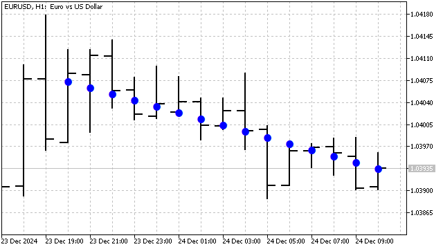
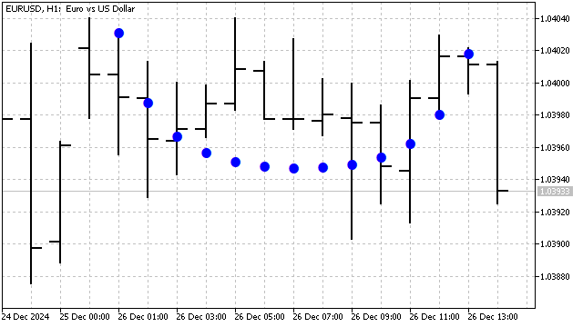
This is the SMA equation. The weights of higher-order polynomials are equivalent to some oscillators with specially selected ratios. In other words, orthogonal polynomials are SMA with some cleverly calculated additions. Legendre polynomials are very robust to noise and perform excellently in sorting applications. For example, the Legendre polynomial of the first degree looks like this.

Chebyshev polynomials can also be used for trend detection and smoothing in addition to Legendre polynomials. There are two types of such polynomials. They differ from each other in their behavior at the edges. The main advantage of these polynomials is their sensitivity to sudden price changes. The equation for these polynomials is very simple:

n	polynomials of the first kind	polynomials of the second kind
0	1	1
1	x	2*x
2	2*x^2-1	4*x^2-1
3	4*x^3-3*x	8*x^3-4*x
4	8*x^4-8*x^2+1	16*x^4-12*x^2+1
5	16*x^5-20*x^3+5*x	32*x^5-32*x^3+6*x
6	32*x^6-48*x^4+18*x^2-1	64*x^6-80*x^4+24*x^2-1
7	64*x^7-112*x^5+56*x^3-7*x	128*x^7-192*x^5+80*x^3-8*x
8	128*x^8-256*x^6+160*x^4-32*x^2+1	256*x^8-448*x^6+240*x^4-40*x^2+1
9	256*x^9-576*x^7+432*x^5-120*x^3+9*x	512*x^9-1024*x^7+672*x^5-160*x^3+10*x

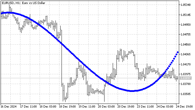
This is what smoothing with the Chebyshev polynomial of the 3rd degree looks like.

So far we have considered polynomials with the definition domain of +/-1, but there are polynomials with other domains. For example, Laguerre polynomial is defined for all non-negative values of the argument. Its equation looks like this:

n	Laguerre polynomials
0	1
1	-x+1
2	(x^2-4*x+2)/2
3	(-x^3+9*x^2-18*x+6)/6
4	(x^4-16*x^3+72*x^2-96*x+24)/24
5	(-x^5+25*x^4-200*x^3+600*x^2-600*x+120)/120
6	(x^6-36*x^5+450*x^4-2400*x^3+5400*x^2-4320*x+720)/720
7	(-x^7+49*x^6-882*x^5+7350*x^4-29400*x^3+52920*x^2-35280*x+5040)/5040
8	(x^8-64*x^7+1568*x^6-18816*x^5+117600*x^4-376320*x^3+564480*x^2-322560*x+40320)/40320
9	(-x^9+81*x^8-2592*x^7+42336*x^6-381024*x^5+1905120*x^4-5080320*x^3+6531840*x^2-3265920*x+362880)/362880

And the shift function for its argument looks like this:

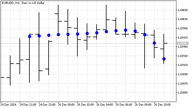
This change leads to the fact that the behavior of the Laguerre polynomial depends not only on the degree, but also on its period. This polynomial is sensitive to recent price changes. For example, this is what the Laguerre polynomial of the fifth degree looks like on a graph:

Another interesting example of orthogonality is Hermite polynomials. These polynomials are used in many areas of math and physics. These polynomials are defined for any values of the argument, and their equation looks like this:

n	Hermite polynomials
0	1
1	x
2	x^2-1
3	x^3-3*x
4	x^4-6*x^2+3
5	x^5-10*x^3+15*x
6	x^6-15*x^4+45*x^2-15
7	x^7-21*x^5+105*x^3-105*x
8	x^8-28*x^6+210*x^4-420*x^2+105
9	x^9-36*x^7+378*x^5-1260*x^3+945*x

The shift function centers the price values:

As a result, we obtained a smoothing filter, the efficiency of which depends on the degree of the polynomial and its period.

We have considered the basic classical orthogonal polynomials. But it is quite possible to create your own version of such polynomials. For example, a polynomial that combines the advantages of the Chebyshev and Hermite polynomials is given by the equation:

n	Chebyshev-Hermite polynomials
0	1
1	2*x
2	4*x^2-2
3	8*x^3-12*x
4	16*x^4-48*x^2+12
5	32*x^5-160*x^3+120*x
6	64*x^6-480*x^4+720*x^2-120
7	128*x^7-1344*x^5+3360*x^3-1680*x
8	256*x^8-3584*x^6+13440*x^4-13440*x^2+1680
9	512*x^9-9216*x^7+48384*x^5-80640*x^3+30240*x

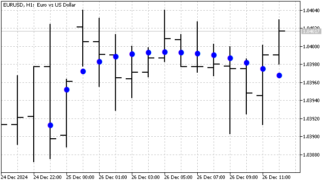
This polynomial is sensitive to nonlinear trends - quadratic, cubic, etc. This is what the Chebyshev-Hermite polynomial of the 9th degree looks like on a graph:

The use of orthogonal polynomials provides a number of advantages.

• Stability and de-correlation. The orthogonality of polynomials ensures their stability to changes in model parameters. Each polynomial is independent of the others, which allows each component of the time series to be modeled and studied separately.
• Interpretability. Each orthogonal polynomial corresponds to its own model of price behavior. The weighting ratios of polynomials allow us to identify the most important models and focus on them.
• Adaptability and efficiency. Orthogonal polynomials are adjusted to specific values of the time series. The emergence of new prices leads to a change in the weighting ratios, due to which the polynomial model adapts to the current state of the market. And the use of nonlinear polynomials makes this adaptation efficient.

The only feature of orthogonal polynomials that can be considered a disadvantage is that these polynomials handle all prices inside the polynomial. In other words, an indicator built on such polynomials "draws". In my opinion, this feature is not a disadvantage - the indicator simply finds the best approximation when new data arrives.

The use of orthogonal polynomials imposes some limitations. The indicator period should be greater than the degree of the polynomial. For practical purposes, we can limit ourselves to the 3rd degree of the polynomial. This indicator combines SMA, linear trend and two parabolas - quadratic and cubic. This is enough to smooth out quite complex situations. But, by increasing the indicator period, we can also increase the degree of the polynomial.

Now, let's look at some examples of the application of orthogonal polynomials in trading.

Trading strategies

Based on orthogonal polynomials, traders can create various trading strategies. For example, using polynomial regression based on orthogonal polynomials, a trader can not only analyze past price movements, but also create a model that can adapt to current changes in the market.

As an example, let's look at several trading strategies based on deviations from the mean.

Let's take the simplest strategy - positions are opened when the price crosses the SMA. We will replace the moving average with an orthogonal polynomial leaving the rules for opening and closing positions unchanged:

• The price crosses the polynomial from bottom to top - open a buy position, close a sell position.
• The price crosses the polynomial from top to bottom - open a sell position, close a buy position.

Despite its simplicity, this strategy is quite efficient.

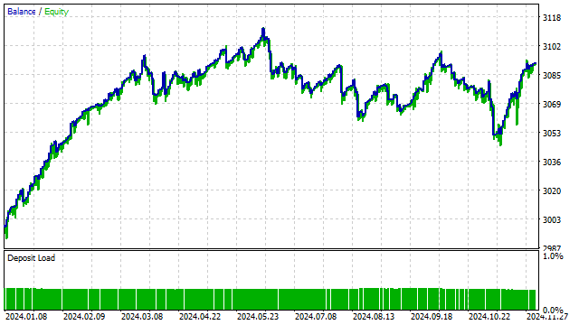
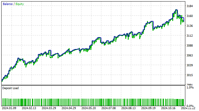
Let's complicate this strategy a little and replace the price with the value of some polynomial. In other words, we will get an analogue of the strategy with the intersection of two SMAs. The result is somewhat predictable: of all possible options, the strategy optimizer preferred orthogonal polynomials.

Polynomial models can also be used in more complex strategies. If the strategy uses any indicators, you can try to replace them with orthogonal polynomials. Such a replacement could improve the strategy.

I will use the Commodity channel index (CCI) indicator as an example. Its classic equation looks like this:

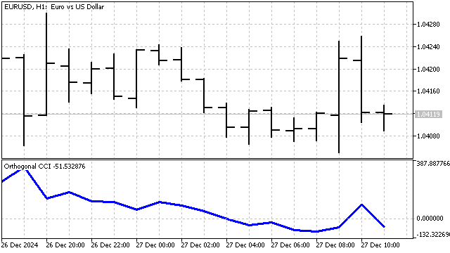
I will make some minor changes to this indicator. As I already said: SMA is a polynomial of degree 0. Instead of SMA, I will use an orthogonal polynomial of any degree. Accordingly, I will calculate the mean absolute deviation relative to this polynomial. The resulting indicator is as follows:

The trading strategy will be similar to the classic one:

• open a buy position if the indicator is below the specified level and continues to decline;
• open a sell position if the indicator is above the specified level and continues to rise;
• close positions on the opposite signal.

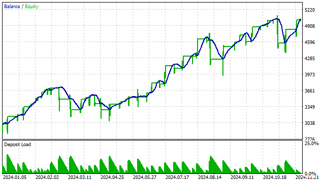
The result of testing such a strategy with a 3rd degree polynomial:

Other indicators can also be constructed based on orthogonal polynomials. For example, I want to construct an equivalent of RSI. The essence is simple: first I build a polynomial, and then I count how many prices were located above this polynomial. Based on this number, I conclude that the price is overbought/oversold.

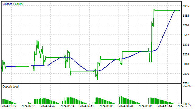
I use the indicator to create a simple strategy:

• open a position if the indicator has reached the overbought or oversold level;
• close positions if the indicator is in the center.

Moreover, orthogonal polynomials can be integrated into various machine learning algorithms. The flexibility of polynomial functions enables machine learning algorithms to detect complex relationships in data. 

For example, polynomials can be used to generate new features from source data. Orthogonal polynomials provide independent estimates of the different components of a time series. Due to this property, they can reduce overfitting. This can improve the quality of training data and improve the performance of models.

Take any neural network and feed the values of the weighting ratios of the orthogonal polynomials to it. But in this case, it will be necessary to construct a complete system of polynomials: starting with a polynomial of the 1st degree, and ending with N-1, where N is the number of prices processed.

Conclusion

Orthogonal polynomials are a powerful tool for analyzing financial time series. They provide a number of benefits and allow us to assess changes in the market. Using orthogonal polynomials in trading strategies can improve their efficiency and enhance trading results.

The following programs were used when writing this article.

Name	Type	Description
Orthogonal polynomials	indicator	simulates orthogonal polynomials on a graph Type - polynomial type iPeriod - polynomial period (not less than 2) N - polynomial degree, acceptable values 0 - 9 Shift - indicator shift
EA Orthogonal polynomials	EA	implements a trading strategy based on the intersection of price and polynomial
EA Orthogonal polynomials 2	EA	implements a strategy at the intersection of two polynomials
Orthogonal CCI	indicator	CCI, in which orthogonal polynomials can be used instead of SMA
EA Orthogonal CCI	EA	implements a strategy based on the orthogonal variant of CCI
Orthogonal RSI	indicator	determines overbought/oversold conditions using orthogonal polynomials
EA Orthogonal RSI	EA	implements a strategy based on the orthogonal version of RSI