Neural Networks in Trading: LSTM Optimization for Multivariate Time Series Forecasting (DA-CG-LSTM)

Introduction

Financial markets are more than just numbers on screens. They are a dynamic environment in which every tick, every candlestick, and every change in trading volume reflects human emotions, expectations, fears, and hopes. Understanding this rhythm and learning to predict where prices will go is a challenge that traders constantly strive to solve.

The focus is on the multivariate time series — the classical representation of market data: asset prices over time, trading volumes, technical indicators, and news flows. All of these are forms of data that can be analyzed, modeled, and ultimately used for forecasting.

Until recently, the industry relied primarily on time-tested classical methods such as ARIMA, SARIMA, and related models. These models are practical, interpretable, and do not require enormous computational resources. They performed reasonably well when dealing with seasonality and linear dependencies, particularly under stable market conditions. However, financial markets are non-stationary. News influences expectations, investor sentiment can shift within seconds, algorithmic trading creates resonance effects, and all of this gives rise to complex, nonlinear, and often chaotic relationships. Traditional models may indicate the general direction, but they fail to capture the finer details.

The emergence of deep learning fundamentally changed this landscape. Recurrent Neural Networks (RNNs) enabled models to account for historical dynamics, yet they were far from a universal solution. Their primary limitation is the so-called "short memory" problem. In other words, such models can process only a limited temporal context. As input sequences become longer, they quickly lose important information from the earlier portions of a time series.

To address this issue, improved architectures such as LSTM (Long Short-Term Memory) and GRU (Gated Recurrent Unit) were developed. These models gave memory to neural networks, i.e., the ability to retain important information over extended time periods.

However, these architectures also have their own limitations. Despite their ability to capture longer-term dependencies, they remain highly sensitive to the quality of the input data. In particular, they struggle with situations where short-term market spikes play a decisive role. Such short-term shifts are often not retained in the model's long-term memory, especially when they are not accompanied by significant changes in the long-term context.

To overcome these shortcomings, the attention mechanism was introduced. It enabled models to focus selectively on the most relevant segments of a time series, regardless of their distance from the current time step. Unlike LSTM, attention mechanisms do not require sequential processing of every temporal step and can immediately concentrate on the most informative elements. This significantly improved the ability of neural networks to capture long-range dependencies, particularly in complex multivariate time series.

However, this approach also has a drawback: such models excel at capturing long-term dependencies but tend to overlook short-term signals that may be critically important. Financial markets do not tolerate delays — a single news headline can send prices soaring or crashing. If a model fails to react to such events, it loses the opportunity to adjust its position in a timely manner.

The authors of the paper "A Dual-Staged Attention Based Conversion-Gated Long Short Term Memory for Multivariable Time Series Prediction" attempted to combine the best of both approaches and proposed a new framework Dual-Staged Attention Conversion-Gated LSTM (DA-CG-LSTM). The model employs a dual attention mechanism. In the first stage, it evaluates the importance of both features and temporal intervals; then, after processing the data through a specialized CG-LSTM block, it re-examines temporal dependencies, amplifying significant signals while suppressing less relevant ones.

An additional advantage of the model lies in its carefully designed activation functions, which improve both long-term information retention and responsiveness to short-term market fluctuations.

The DA-CG-LSTM Algorithm

The DA-CG-LSTM framework is designed to extract meaningful patterns from multivariate time series. Its architecture combines two layers of attention with a modified recurrent block known as Conversion-Gated LSTM. This makes the model particularly effective for forecasting dynamic multivariate processes.

The process begins by feeding a multivariate temporal sequence into the model. This sequence is represented by the matrix X = [x1, x2, ..., xT] ∈ RT*n, where each row xt is a vector of n features at time t. However, the model does not process this information blindly. It first learns to identify which features and which time steps are genuinely important. This is how the first stage begins: input attention.

Initially, the model analyzes the features within each individual time step. It computes the importance score of each feature xkt at time step t according to the following formula:

Here We and be denote the trainable weights and biases of a linear layer applied to each input feature vector xt. This layer transforms the raw data into a more informative latent representation suitable for relevance estimation. In addition, the trainable vector ve serves as an interpretable attention mask used to compute a scalar importance score. This design allows the model to flexibly rank features according to their contribution, which is particularly valuable when dealing with noisy, high-dimensional time series.

The resulting importance coefficients are normalized using the SoftMax function, transforming the set of scores into a probability distribution over the features:

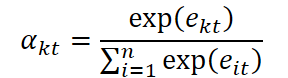
These coefficients are then used to adjust the original input vector x ̃t with each feature scaled according to its estimated importance.

But we do not stop there. In the next step, the model evaluates the importance of each temporal position, determining which points in time should be emphasized during processing. A similar structure is applied:

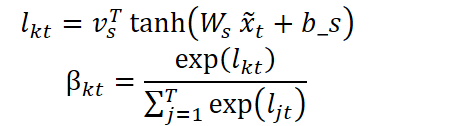
The resulting sequence is a time-weighted representation:

Thus, even before recurrent processing begins, the model has already concentrated its attention on the information it considers most relevant.

The sequence is then passed into the modified recurrent block, CG-LSTM. Here the second stage of the process takes place. Within the standard LSTM architecture, the authors redesigned the activation functions associated with the input and forget gates. This was done to increase the model's sensitivity to short-term spikes accompanying short-term market shifts, while simultaneously strengthening its ability to remember long-term information.

In a conventional LSTM block, the input gate relies on the sigmoid activation function to determine which information should be retained. However, sigmoid functions are prone to saturation: when input values become very small or very large, their derivatives approach zero, reducing learning efficiency. The authors of the DA-CG-LSTM framework proposed combining the sigmoid function with the hyperbolic tangent function, expressed by the following formula:

This design helps prevent saturation during the early stages of training while preserving sensitivity to subtle but meaningful fluctuations. In financial time series, this capability is particularly important. For example, a sudden increase in trading volume or a spike in volatility may indicate a regime shift in the market, and the timely detection of such patterns provides a significant forecasting advantage.

The forget gate in CG-LSTM was also modified. Unlike the standard LSTM architecture, it employs a function that combines the sigmoid function with a transformed hyperbolic tangent expression:

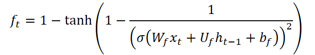
This formulation possesses a distinctive property: its derivative ranges from 0 to approximately 2.89, producing a data dispersion effect. In practice, this enables the model to discard irrelevant or outdated information more aggressively, thereby focusing on recent developments. This property is especially valuable in financial markets, where historical events rapidly lose relevance and success often depends on reacting to current signals.

The output of the CG-LSTM block is the sequence (h1, h2, ..., hT), where each ht contains both short-term and long-term information. However, retaining information alone is insufficient — it must also be recalled correctly. This is the purpose of the second attention layer: temporal attention.

At this stage, the model effectively re-examines its own memory. It computes the importance of each hidden state hj relative to the current time step. The resulting values are normalized using SoftMax, and a context vector is constructed — a distilled essense of the entire temporal history — which is subsequently processed by a second CG-LSTM block.

Using the current hidden state ht together with the enriched context ct, the model produces its final forecast:

where f is typically a fully connected layer or another output component of the architecture.

The DA-CG-LSTM architecture is not merely intelligent; it is sensible. The model does not memorize everything. Instead, it makes informed choices. It does not react to every instance of noise but learns to distinguish transient fluctuations from meaningful patterns. This distinction is particularly important in financial forecasting. The system can identify signals analogous to those observed in the past, assess their significance, and adjust its predictions.

In this sense, DA-CG-LSTM functions as a dynamic, adaptive system that learns, evolves, and draws conclusions through structured information analysis. Its strength lies not only in its mathematical formulations but also in its conceptual clarity:

Attention + Memory + Interpretation = Meaningful Forecasting

The author's visualization of the DA-CG-LSTM framework is presented below.

Implementation in MQL5

Having examined the theoretical aspects of the DA-CG-LSTM framework, we now move on to the practical part of this work, where we will present our own implementation of the proposed approach using MQL5.

We will begin by constructing a modified CG-LSTM block, illustrated below in the author's diagram.

It is important to note that, similarly to a conventional LSTM block, the input tensor is concatenated with the hidden state generated during the previous time step. The resulting tensor is then used to construct four entities: three gates and a new context representation. Each of these entities is produced by a separate linear layer. However, nonlinear behavior is introduced by applying different activation functions to the outputs of these layers.

Using four distinct activation functions for the individual entities would naturally require four fully connected layers executed sequentially. Clearly, this is not an optimal solution. Throughout our work, we strive to maximize operational parallelism, as this accelerates both model training and decision-making under real-world conditions.

To achieve this, when implementing the classical LSTM block, we organized the entire feed-forward pass within a single kernel. The values of each entity were computed simultaneously in parallel workgroup threads, with intermediate values exchanged via local memory. This approach proved highly efficient. However, when using the more complex activation function sequences proposed by the authors of the DA-CG-LSTM framework, we encounter the need for additional data buffers to store intermediate values, which significantly complicates the algorithm.

Therefore, in this implementation, we decided to use an alternative approach. The feed-forward pass is divided into two stages. In the first stage, all four entities are generated without applying activation functions. This can be accomplished using either a fully connected layer or a convolutional layer whose output tensor size is proportional to the number of generated entities. When working with multidimensional input data, a convolutional layer is preferable because it enables independent operations for individual univariate sequences.

The second stage performs the actual CG-LSTM computations by applying the required activation functions and executing the internal processes of the block.

Naturally, we will begin by implementing the second stage within the OpenCL context.

Modifying the OpenCL Program

First, we implement the feed-forward pass of our CG-LSTM block version within the CSLSTM_FeedForward kernel. This kernel receives pointers to only three data buffers.

One of these buffers contains the input data (concatenated), which stores the values of the four components before activation functions are applied. To minimize latency associated with global memory access and improve read performance, the values are stored using the float4 vector type, allowing four consecutive elements to be fetched with a single memory access. This organization makes more efficient use of memory bandwidth and accelerates computations, especially when processing large volumes of input data.

The remaining two buffers are used to store the context and output values.

__kernel void CSLSTM_FeedForward(__global const float4* __attribute__((aligned(16))) concatenated,
                                 __global float *memory,
                                 __global float *output)
  {
   uint id = (uint)get_global_id(0);
   uint total = (uint)get_global_size(0);       // hidden size
   uint idv = (uint)get_global_id(1);
   uint total_v = (uint)get_global_size(1);     // variables

This kernel operates within a two-dimensional execution space without creating workgroups. The first dimension corresponds to the size of the cell's hidden state, while the second dimension represents the number of univariate sequences in the input data. In the kernel body, we identify the thread in all dimensions of the task space.

Using this information, we determine the appropriate offsets in the data buffers and immediately load the corresponding block of input data into a local variable.

uint shift = id + total * idv;
float4 concat = concatenated[shift];

Next, we apply the required activation functions to all entities.

float fg = 1 - Activation(1 - 1 / pow(Activation(concat.s0, ActFunc_SIGMOID), 2), ActFunc_TANH);
float ig = Activation(Activation(concat.s1, ActFunc_SIGMOID), ActFunc_TANH);
float nc = Activation(concat.s2, ActFunc_TANH);
float og = Activation(concat.s3, ActFunc_SIGMOID);

Afterward, we update both the context values and the hidden state.

float mem = IsNaNOrInf(memory[shift] * fg + ig * nc, 0);
float out = IsNaNOrInf(og * Activation(mem, ActFunc_TANH), 0);

The resulting values are saved in the corresponding elements of the global data buffers, after which the kernel execution is completed.

 memory[shift] = mem;
 output[shift] = out;
} 

The resulting kernel code is compact and easy to read, largely thanks to the use of a helper method responsible for selecting activation functions. This approach not only simplifies the logic of the kernel itself but also makes the code more modular and extensible. In addition, incorporating a mechanism for validating computed values improves the reliability of the entire computational pipeline.

After completing the feed-forward kernel, we proceed to implement the backpropagation operations. It is easy to see that no trainable parameters are used during the feed-forward pass. All trainable parameters are placed in the neural layer used during the first stage. Therefore, implementing backpropagation only requires us to correctly distribute the error gradients among the participating components. These operations are performed inside the CSLSTM_CalcHiddenGradient kernel.

The parameters of the gradient-distribution kernel are supplemented with the appropriate data buffers, while preserving the original execution space.

__kernel void CSLSTM_CalcHiddenGradient(__global const float4* __attribute__((aligned(16))) concatenated,
                                        __global float4* __attribute__((aligned(16))) grad_concat,
                                        __global const float* memory,
                                        __global const float* grad_output
                                       )
  {
   uint id = get_global_id(0);
   uint total = get_global_size(0);
   uint idv = get_global_id(1);
   uint shift = id + total * idv;

In the kernel body, we identify the current thread across all dimensions and immediately calculate the corresponding offsets in the data buffers.

It should be noted that computing the derivatives of the complex activation functions proposed by the DA-CG-LSTM framework requires several intermediate values that were intentionally not saved during the feed-forward pass. Clearly, saving these values would have required substantial memory resources. Moreover, accessing global data buffers is an expensive operation. However, because the bulk of the matrix computations was delegated to the internal neural layer of the first stage, we can quickly compute the required values from the pre-activation entity values.

To achieve this, we read the pre-activation data into local variables and recompute the functions, saving intermediate results locally. 

   float4 concat = concatenated[shift];                    // Pre-activation values for all 4 gates
// --- Forward reconstruction of gates ---
   float fg_s = Activation(concat.s0, ActFunc_SIGMOID);
   float fg = 1.0f - Activation(1.0f - 1.0f / pow(fg_s, 2), ActFunc_TANH);  // Forget gate (ft)
   float ig_s = Activation(concat.s1, ActFunc_SIGMOID);
   float ig = Activation(ig_s, ActFunc_TANH);              // Input gate (it)
   float nc = Activation(concat.s2, ActFunc_TANH);         // New content (ct~)
   float og = Activation(concat.s3, ActFunc_SIGMOID);      // Output gate (ot)
   float mem = memory[shift];                              // New memory state (ct)
   float mem_t = Activation(mem, ActFunc_TANH);            // tanh(ct)

At this stage, we also reconstruct the memory state from the previous time step.

// --- Reconstruct previous memory state (t-1) ---
   float prev_mem = IsNaNOrInf((mem - ig * nc) / fg, 0);

After completing the preparatory computations, we proceed directly to the gradient-distribution operations. First, we load the output gradient from the global buffer into a local variable.

// --- Gradients computation ---
   float out_g = grad_output[shift];

Next, we distribute this gradient between the output gates and the context memory using the derivatives of the corresponding activation functions.

float og_g = Deactivation(out_g * mem_t, og, ActFunc_SIGMOID);
float mem_g = Deactivation(out_g * og, mem_t, ActFunc_TANH);

Then we propagate the context memory gradient between the new context projection and the input gates.

float nc_g = Deactivation(mem_g * ig, nc, ActFunc_TANH);
float ig_g = Deactivation(Deactivation(mem_g * nc, ig, ActFunc_TANH), ig_s, ActFunc_SIGMOID);

Particular attention should be paid to the stages involving the derivatives of the respective activation functions, which are applied sequentially while updating the gradients of the input gates.

Finally, we propagate the error gradient down to the forget gate values prior to activation. As mentioned earlier, the authors of the DA-CG-LSTM framework proposed a relatively complex activation function for this component. Consequently, gradient propagation must be performed in several stages.

First, we determine the forget gate error based on the context memory gradient and its previous value.

// ∂L/∂fg = ∂L/∂ct * mem_(t-1)
   float fg_g = mem_g * prev_mem;

The resulting value is then adjusted using the derivative of the hyperbolic tangent function and the derivative of the complex internal expression.

// Derivative of the complex forget gate:
// f(z) = 1 - tanh(1 - 1 / σ(z)^2)
   float fg_s_g = 2 / pow(fg_s, 3) * Deactivation(-fg_g, fg, ActFunc_TANH);
   fg_g = Deactivation(fg_s_g, fg_s, ActFunc_SIGMOID);

Finally, we apply the sigmoid derivative.

The resulting values are stored in the corresponding locations of the global data buffer.

// --- Write back gradients ---
   grad_concat[shift] = (float4)(fg_g, ig_g, nc_g, og_g);
  }

This concludes our work on the OpenCL-side implementation. The complete source code is provided in the attachment.

Creating the CG-LSTM Object

Next, we move to the main program. Here, we create a new object, CNeuronCGLSTMOCL, responsible for managing the operation of our CG-LSTM block. The structure of the new object is presented below.

class CNeuronCGLSTMOCL : public CNeuronBaseOCL
  {
protected:
   CNeuronBaseOCL    cConcatenateInputs;
   CNeuronConvOCL    cProjection;
   //---
   virtual bool      CSLSTM_feedForward(void);
   virtual bool      CSLSTM_CalcHiddenGradient(void);
   //---
   virtual bool      feedForward(CNeuronBaseOCL *NeuronOCL) override;
   virtual bool      updateInputWeights(CNeuronBaseOCL *NeuronOCL) override;
   virtual bool      calcInputGradients(CNeuronBaseOCL *NeuronOCL) override;

public:
                     CNeuronCGLSTMOCL(void) {};
                    ~CNeuronCGLSTMOCL(void) {};
   //---
   virtual bool      Init(uint numOutputs, uint myIndex, COpenCLMy *open_cl, uint numNeurons,
                          ENUM_OPTIMIZATION optimization_type, uint batch) override;
   virtual bool      Init(uint numOutputs, uint myIndex, COpenCLMy *open_cl,
                          uint count, uint window, uint variables, 
                          ENUM_OPTIMIZATION optimization_type, uint batch);
   //---
   virtual bool      Save(int const file_handle) override;
   virtual bool      Load(int const file_handle) override;
   //---
   virtual int       Type(void) override  const    {  return defNeuronCGLSTMOCL; }
   virtual bool      Clear(void) override;
   virtual CBufferFloat *getLSTMWeights(void) { return cProjection.GetWeightsConv(); }
   virtual void      SetOpenCL(COpenCLMy *obj) override;
   virtual bool      WeightsUpdate(CNeuronBaseOCL *source, float tau) override;
  };

In the new class structure, we see a familiar set of overridden methods and two internal objects, whose functionality will become clearer as we implement the class methods. All internal objects are declared directly as class members, allowing us to keep the class constructor and destructor empty. The initialization of the declared and inherited objects is performed inside the Init method.

The initialization method receives a number of constants that uniquely define the architecture of the object being created.

bool CNeuronCGLSTMOCL::Init(uint numOutputs, uint myIndex, COpenCLMy *open_cl,
                            uint count, uint window, uint variables,
                            ENUM_OPTIMIZATION optimization_type, uint batch)
  {
   if(!CNeuronBaseOCL::Init(numOutputs, myIndex, open_cl, count * variables, optimization_type, batch))
      return false;
   SetActivationFunction(None);

Part of these values is immediately passed to the identically named method of the parent class, which already handles parameter validation and the initialization of inherited objects.

Note that we explicitly specify the absence of an activation function for the newly created object.

After the parent-class initialization completes successfully, we proceed to preparing the declared objects for operation. In this case, there are only two. The first is a fully connected layer used to store the concatenated tensor consisting of the input data and the hidden state generated during previous feed-forward passes.

if(!cConcatenateInputs.Init(0, 0, OpenCL, (count + window) * variables, optimization, iBatch))
   return false;
cConcatenateInputs.SetActivationFunction(None);

Again, we explicitly indicate the absence of the activation function.

The second object is a convolutional layer responsible for projecting the concatenated tensor into four entities.

if(!cProjection.Init(0, 1, OpenCL, count + window, count + window, count * 4, 1, variables, optimization, iBatch))
   return false;
cProjection.SetActivationFunction(None);

As discussed earlier, this layer also operates without an activation function, which we explicitly specify.

Special attention should be paid to the initialization of the convolutional layer. During its creation, we explicitly set the sequence length to one. At first glance, this may appear restrictive; however, this design choice reflects a deliberate architectural decision. At the same time, we specify the number of univariate (independent) sequences that will be processed in parallel.

This approach allows each univariate sequence to maintain its own independent set of trainable parameters — its own weight matrix. As a result, each sequence can be analyzed and trained independently. Each sequence learns within its own context, responding to specific patterns and regularities without sharing parameters with other sequences. Consequently, we obtain a more expressive, more adaptive, and structurally flexible representation of the input data, especially in tasks where different temporal subsequences serve distinct semantic functions or represent individual market factors.

Such parameter isolation also plays an important role during training. First, it reduces cross-interference between channels, thereby mitigating overfitting to dominant patterns. Second, each unitary sequence can focus on its own data characteristics. This type of differentiated learning makes the model not only more accurate for specific tasks but also significantly more robust to changing market conditions.

Furthermore, independently trained univariate filters promote better generalization. The model becomes less prone to memorizing data and more likely to extract general patterns. This is particularly important for financial time series, where historical data may contain unique, non-representative events. By decomposing the learning process into multiple isolated branches, the model becomes capable of recognizing typical market signals even in previously unseen situations.

Finally, one of the defining characteristics of recurrent models is their reliance on data from the previous feed-forward pass. Therefore, we clear all data buffers before completing the initialization process.

   if(!Clear())
      return false;
//---
   return true;
  }

The next stage of our work is the implementation of the forward-pass operations, which we implement in the feedForward method. This part is relatively straightforward. The method receives a pointer to the input data object, which is immediately validated.

bool CNeuronCGLSTMOCL::feedForward(CNeuronBaseOCL *NeuronOCL)
  {
   if(!NeuronOCL)
      return false;

Next, we extract the dimensions of both the input tensor and the hidden state from the projection layer parameters.

int hidden = (int)cProjection.GetFilters() / 4;
int inputs = (int)cProjection.GetWindow() - hidden;
int variables = (int)cProjection.GetVariables();

We then concatenate the input data with the results of the previous feed-forward pass for each univariate sequence.

if(!Concat(NeuronOCL.getOutput(), getOutput(), cConcatenateInputs.getOutput(), inputs, hidden, variables))
   return false;

The resulting values are projected into four entities.

if(!cProjection.FeedForward(cConcatenateInputs.AsObject()))
   return false;

At this point, all that remains is to call the wrapper method that enqueues the previously created feed-forward kernel CSLSTM_feedForward for execution.

 return CSLSTM_feedForward();
}

The methods for placing kernels in the execution queue follow the same architecture discussed in previous articles, so we will not examine their internal algorithm in detail here.

Having completed the feed-forward implementation, we move on to the backpropagation procedures. As you know, this process consists of two stages: distributing the error gradients and optimizing the trainable parameters.

In this case, the trainable parameters exist only within the projection layer of the concatenated data. Therefore, parameter optimization is reduced to calling the corresponding optimization method of the projection layer.

bool CNeuronCGLSTMOCL::updateInputWeights(CNeuronBaseOCL *NeuronOCL)
  {
   return cProjection.UpdateInputWeights(cConcatenateInputs.AsObject());
  }

The algorithm for distributing error gradients among participating components, implemented in calcInputGradients, is slightly more complex. The method receives a pointer to the input data object. This is the same object used during the feed-forward pass. However, this time, we must propagate the error gradient into it according to the contribution of the input data to the model's final output.

bool CNeuronCGLSTMOCL::calcInputGradients(CNeuronBaseOCL *NeuronOCL)
  {
   if(!NeuronOCL)
      return false;

In the method body, we immediately verify the validity of the received pointer. The necessity of this control point has been discussed repeatedly in previous articles.

Next, similarly to the feed-forward method, we determine the dimensions of the input data and the hidden state.

int hidden = (int)cProjection.GetFilters() / 4;
int inputs = (int)cProjection.GetWindow() - hidden;
int variables = (int)cProjection.GetVariables();

We begin by distributing the error gradient among the entities by calling the wrapper method that places the corresponding kernel in the execution queue.

if(!CSLSTM_CalcHiddenGradient())
   return false;

Then, we propagate the gradient down to the concatenated input tensor.

if(!cConcatenateInputs.calcHiddenGradients(cProjection.AsObject()))
   return false;

Using reverse concatenation, we extract the error gradient corresponding to the original input data.

if(!DeConcat(NeuronOCL.getGradient(), getPrevOutput(), cConcatenateInputs.getGradient(),
                                                             inputs, hidden, variables))
   return false;

It is worth noting that, during the initialization of the internal objects, we intentionally disabled activation functions. However, this does not exclude the use of activation functions within the input data itself. Therefore, we check whether an activation function is associated with the input data and, if necessary, adjust the resulting gradients using the derivatives of the corresponding activation functions.

   if(NeuronOCL.Activation() != None)
      if(!DeActivation(NeuronOCL.getOutput(), NeuronOCL.getGradient(), NeuronOCL.getGradient(),
                                                                       NeuronOCL.Activation()))
         return false;
//---
   return true;
  }

We then complete the method by returning the logical result of the operation to the caller.

This concludes our examination of the algorithms used to construct the methods of the new CNeuronCGLSTMOCL class. The complete source code for this class and all of its methods is available in the attachments.

Gradually, almost without noticing it ourselves, we have reached the practical limits of the current article. However, the logical completion of this research requires a continuation. We will pause here for now. To be continued — and the next part will be no less substantial. 

Conclusion

In this article, we examined the theoretical foundations of the DA-CG-LSTM framework. Unlike traditional models, its architecture incorporates several innovative mechanisms, including CG-LSTM and a dual-attention mechanism, both of which enable deeper and more accurate extraction of dependencies from data. These components allow the model to effectively process complex temporal relationships while simultaneously capturing both long-term and short-term patterns.

In the practical section, we presented our own implementation of the CG-LSTM block using MQL5. However, this work is not yet complete, and we will continue it in the next article, bringing the project to its logical conclusion.

References

• A Dual-Staged Attention Based Conversion-Gated Long Short Term Memory for Multivariable Time Series Prediction
• Other articles from this series

Programs Used in This Article

#	Name	Type	Description
1	Research.mq5	Expert Advisor	Expert Advisor for collecting samples
2	ResearchRealORL.mq5	Expert Advisor	Expert Advisor for collecting samples using the Real-ORL method
3	Study.mq5	Expert Advisor	Expert Advisor for offline model training
4	StudyOnline.mq5	Expert Advisor	Expert Advisor for online model training
4	Test.mq5	Expert Advisor	Expert Advisor for model testing
5	Trajectory.mqh	Class library	System state and model architecture description structure
6	NeuroNet.mqh	Class library	A library of classes for creating a neural network
7	NeuroNet.cl	Code library	OpenCL program code