Generative Adversarial Networks (GANs) for Synthetic Data in Financial Modeling (Part 1): Introduction to GANs and Synthetic Data in Financial Modeling

Algorithmic trading relies on quality financial data, but issues like small or unbalanced samples can harm model reliability. Generative Adversarial Networks (GANs) offer a solution by generating synthetic data, enhancing dataset diversity and model robustness.

GANs, introduced in 2014 by Ian Goodfellow, are machine learning models that simulate data distributions to create realistic copies, widely used in finance to address data scarcity and noise. For example, GANs can generate synthetic stock price sequences, enriching limited datasets for better generalization in models. However, training GANs is computationally demanding, and synthetic data should be carefully validated for relevance to avoid mismatches with real market conditions.

The structure of a GAN

GANs are simply the two neural networks - the Generator and the Discriminator-that play an adversarial game: Here's a breakdown of these components. 

• Generator: By the word Generator, the intent here is to train an algorithm to mimic actual data. It works with random noise as an input and over time tends to produce data samples that are more realistic. In trading terms, the Generator would give out fake price movement or trading volume sequences that resemble real sequences. 

• Discriminator: The role of the Discriminator is to decide which data out of the structured data and synthesized data is genuine. Each data sample is then assessed on its likelihood of being original data or synthesized data. As a result, in a training process, the Discriminator increases in ability to classify the input as real data, thus encouraging the Generator to advance in generating the data.

Let's now look at the Adversarial process since it is the very adversarial aspect of GANs that makes them so powerful. Here's how the two networks interact during the training process:

• Step 1: The Generator creates a batch of synthetic data samples through noise. 
• Step 2: The Discriminator takes in the real data as well as the Synthetic data from the Generator. It assigns possibilities, or in other words it "passes judgment" in the authenticity of each sample. 
• Step 3: In the next interactions, based on the Discriminator's feedback, the weight of the Generator is adjusted to generate more realistic data. 
• Step 4: The discriminator also changes its weight to better distinguish real data from fake data. 

This ongoing cycle continues until the Generator's Synthetic data is highly accurate and can no longer be distinguished by the Discriminator from the real data. At this point, the GAN is considered trained since the Generator is generating Synthetic data of great quality. 

The loss of the Generator reduces as it comes closer to generating more realistic data and the loss of the Discriminator varies as and when the Discriminator tries to adapt to the Generator's improved output. 

Here’s a simplified structure for a GAN in Python using TensorFlow to illustrate how the Generator and Discriminator interact:

import tensorflow as tf
from tensorflow.keras import layers

# Define the Generator model
def build_generator():
    model = tf.keras.Sequential([
        layers.Dense(128, activation='relu', input_shape=(100,)),
        layers.Dense(256, activation='relu'),
        layers.Dense(512, activation='relu'),
        layers.Dense(1, activation='tanh') # Output size to match the data shape
    ])
    return model

# Define the Discriminator model
def build_discriminator():
    model = tf.keras.Sequential([
        layers.Dense(512, activation='relu', input_shape=(1,)),
        layers.Dense(256, activation='relu'),
        layers.Dense(128, activation='relu'),
        layers.Dense(1, activation='sigmoid') # Output is a probability
    ])
    return model

# Compile GAN with Generator and Discriminator
generator = build_generator()
discriminator = build_discriminator()

# Combine the models in the adversarial network
discriminator.compile(optimizer='adam', loss='binary_crossentropy', metrics=['accuracy'])
gan = tf.keras.Sequential([generator, discriminator])
gan.compile(optimizer='adam', loss='binary_crossentropy')

In this structure:

The generator transforms random noise into realistic synthetic data, then the Discriminator classifies the input as real or fake, and the GAN combines both models, enabling them to learn from each other iteratively.

Training a GAN

So far we have known the structure of a GAN we can now move to the training of a GAN which is an interactive process, where the Generator and Discriminator networks are trained simultaneously in turn to improve their performance. The training process is a series of steps in which each of the networks performs in a way that the other can learn from, making it possible for them to offer enhanced results. Now we will discuss the main parts of the process of training an effective GAN. The core of the GAN training is an alternative, two-step process where each network is updated independently in each cycle :

• Step 1: Train the Discriminator. 

First, the Discriminator receives real data samples and estimates the probability of each of them being real, then it receives Synthetic data generated by the Generator. Next, the loss of the Discriminator is determined by its capacity to classify the real and Synthetic samples. Its weights are adjusted to minimize this loss, improving its capacity to identify real data from fake.

•  Step 2: Train the Generator. 

The Generator generates synthetic samples from random noise and then takes them to the Discriminator. Then Discriminator's predictions are used to compute the Generator loss because the Generator "wants" the Discriminator to say that it was generating realistic data. The weights of the generator are adjusted to reduce its loss so that it can generate more realistic data that would fool the Discriminator.

This process of alternating between each other's predictions is done over and over many times with the networks gradually adapting to each other's changes. 

 The following code demonstrates the core of a GAN training loop in Python using TensorFlow:

import numpy as np
import tensorflow as tf
from tensorflow.keras import layers, Model
from tensorflow.keras.optimizers import Adam

tf.get_logger().setLevel('ERROR')  # Only show errors

# Generator model
def create_generator():
    input_layer = layers.Input(shape=(100,))
    x = layers.Dense(128, activation="relu")(input_layer)
    x = layers.Dense(256, activation="relu")(x)
    x = layers.Dense(512, activation="relu")(x)
    output_layer = layers.Dense(784, activation="tanh")(x)
    model = Model(inputs=input_layer, outputs=output_layer)
    return model

# Discriminator model
def create_discriminator():
    input_layer = layers.Input(shape=(784,))
    x = layers.Dense(512, activation="relu")(input_layer)
    x = layers.Dense(256, activation="relu")(x)
    output_layer = layers.Dense(1, activation="sigmoid")(x)
    model = Model(inputs=input_layer, outputs=output_layer)
    return model

# GAN model to combine generator and discriminator
def create_gan(generator, discriminator):
    discriminator.trainable = False  # Freeze discriminator during GAN training
    gan_input = layers.Input(shape=(100,))
    x = generator(gan_input)
    gan_output = discriminator(x)
    gan_model = Model(inputs=gan_input, outputs=gan_output)
    return gan_model

# Function to train the GAN
def train_gan(generator, discriminator, gan, data, epochs=10000, batch_size=64):
    half_batch = batch_size // 2
    for epoch in range(epochs):
        # Train Discriminator
        noise = np.random.normal(0, 1, (half_batch, 100))
        generated_data = generator.predict(noise, verbose=0)

        real_data = data[np.random.randint(0, data.shape[0], half_batch)]

        # Train discriminator on real and fake data
        d_loss_real = discriminator.train_on_batch(real_data, np.ones((half_batch, 1)))
        d_loss_fake = discriminator.train_on_batch(generated_data, np.zeros((half_batch, 1)))
        d_loss = 0.5 * np.add(d_loss_real, d_loss_fake)

        # Train Generator
        noise = np.random.normal(0, 1, (batch_size, 100))
        g_loss = gan.train_on_batch(noise, np.ones((batch_size, 1)))

        # Print progress every 100 epochs
        if epoch % 100 == 0:
            print(f"Epoch {epoch} | D Loss: {d_loss[0]:.4f} | G Loss: {g_loss[0]:.4f}")

# Prepare data
data = np.random.normal(0, 1, (1000, 784))

# Initialize models
generator = create_generator()
discriminator = create_discriminator()
discriminator.compile(optimizer=Adam(), loss="binary_crossentropy", metrics=["accuracy"])
gan = create_gan(generator, discriminator)
gan.compile(optimizer=Adam(), loss="binary_crossentropy")

# Train GAN
train_gan(generator, discriminator, gan, data, epochs=10000, batch_size=64)

This code trains the Discriminator basically with actual data from the given dataset as well as with the fake/recreated data by the actual Generator. The Real data is classified as ‘1 ’ while the generated Data is classified as ‘0 ’ in training the Discriminator. Then Generator is trained from the Discriminator through a feedback system in a way that the Generator will be creating data that is real-like.

From the Discriminator’s response, the Generator can further hone its ability to create realistic data. The code also prints out losses for the Discriminator and the Generator every one hundred epochs as will be discussed later. This forms a means by which the training progress of the GAN can be evaluated and an assessment made on how well each part of the GAN is performing its intended function at any particular time.

GANs in Financial Modeling

GANs have become quite useful for financial modeling, especially in generating new data. In financial markets, the lack of data or data privacy issues means that high-quality data for training and testing the predictive models is scarce. GANs help solve this issue since they produce synthetic data that have similar statistics as the actual financial datasets.

One of the areas of application we can identify is the field of risk assessment where GANs can model extreme market conditions and help to stress test portfolios without using historical data. Furthermore, GANs are useful in increasing model robustness by generating diverse training data sets thus avoiding overfitting the model. They are also used for outlier generation where complex models are developed to create synthetic datasets that point to such outliers as fraud transactions or market anomalies.

Overall, the use of GANs in financial modeling allows institutions to address the issues of low data quality, simulate the occurrence of events that are not often observed, and increase the predictive power of models, which makes GANs important tools for modern financial analysis and decision-making.

Implementing a Simple GAN in MQL5

Now that we are familiar to the GAN let's move to the generation of synthetic data as a result of training a Generative Adversarial Network (GAN) in MQL5 which offers a novel way of approaching the concept of synthetic data within the trading context. A basic GAN comprises two components: a generator which generates fake data (for instance, price trends) and a discriminator which determines if a data point is genuine or fake. This is how we can apply a simple GAN in MQL5 to model artificial closing prices that mimic the real market dynamics.

• Defining the Generator and Discriminator

The generator generates fake price levels while the discriminator determines how close the data is to actual historical prices. Here’s a basic structure in MQL5:

double GenerateSyntheticPrice() {
    return NormalizeDouble(MathRand() / 1000.0, 5); // Simple random price
}

double Discriminator(double price, double threshold) {
    if (MathAbs(price - threshold) < 0.001) return 1; // Real
    return 0; // Fake
}

The presented example of using GANs in MQL5 shows how one can use them to create synthetic data for financial modeling and testing and thus expand the horizons of improving trading algorithms.

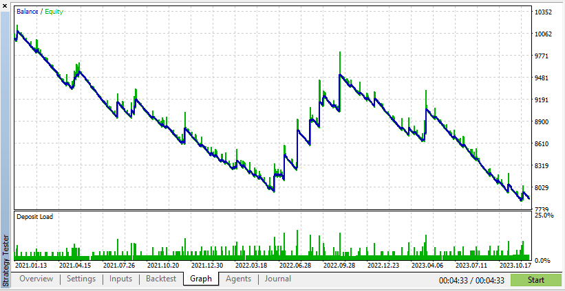
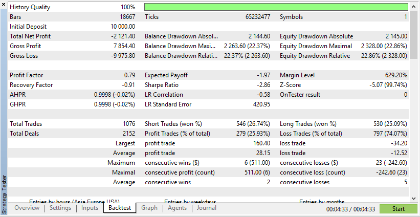
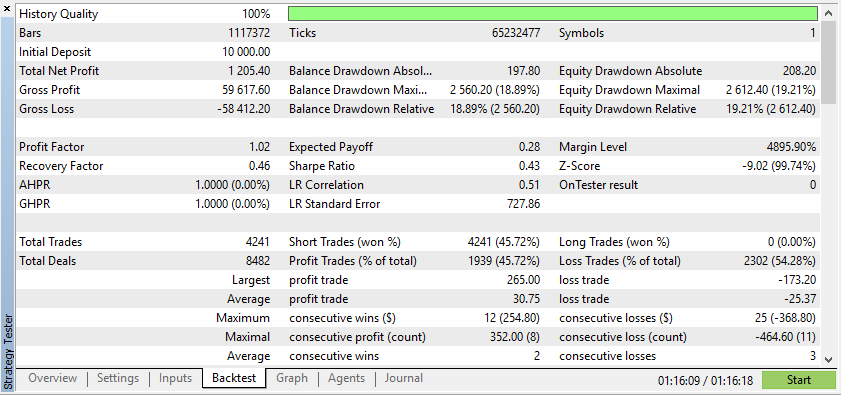
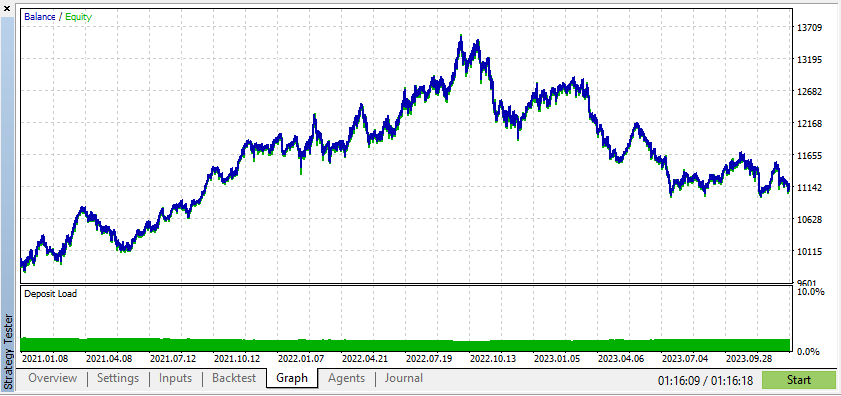
Below is the test for one expert advisor on both real and synthetic data:

According to these results, Real Data has resulted in more realistic, but potentially lower, profits due to the unpredictable nature of actual market conditions.

According to these results, Synthetic Data has shown show higher profits if the data is due to the ideal conditions for your EA.

  

However, real data will give you a much clearer understanding of how the EA will perform under actual trading conditions. Relying on synthetic data can often lead to misleading backtest results, which might not be reproducible in a live market.

Perception of the training of GANs is crucial since it provides insights into the learning process and the stability of the model. In financial modeling, visualization is used to help the modelers understand if the synthetic data has the right pattern like real data as captured by the GAN. The generated outputs in different training stages can be displayed to the developers to detect possible problems such as mode collapse or poor quality of the synthetic data. Such an evaluation is continuous, which enables training to set parameters appropriately while promoting GAN performance for generating data that reflects the target financial patterns.

Below is a code of how you create a synthetic instrument based on 3 years of  EURUSD data:

import pandas as pd
import numpy as np
import matplotlib.pyplot as plt
import os

# Download data using the terminal 
# Replace 'your-api-key' with an actual API key from a data provider
# Here, we simulate this with a placeholder for clarity
api_key = "your-api-key"
symbol = "EURUSD"
output_csv = "EURUSD_3_years.csv"

# Command to download the data from Alpha Vantage or any similar service
# Example using Alpha Vantage (Daily FX data): https://www.alphavantage.co
command = f"curl -o {output_csv} 'https://www.alphavantage.co/query?function=FX_DAILY&from_symbol=EUR&to_symbol=USD&outputsize=full&apikey={api_key}&datatype=csv'"
os.system(command)

# Read the downloaded CSV file
data = pd.read_csv(output_csv)

# Ensure the CSV is structured correctly for further processing
# Rename columns if necessary to match yfinance format
data.rename(columns={"close": "Close"}, inplace=True)

# Print the first few rows to confirm
print(data.head())

# Extract the 'Close' prices from the data
prices = data['Close'].values

# Normalize the prices for generating synthetic data
min_price = prices.min()
max_price = prices.max()
normalized_prices = (prices - min_price) / (max_price - min_price)

# Example: Generating some mock data
def generate_real_data(samples=100):
    # Real data following a sine wave pattern
    time = np.linspace(0, 4 * np.pi, samples)
    data = np.sin(time) + np.random.normal(0, 0.1, samples)  # Add some noise
    return time, data

def generate_fake_data(generator, samples=100):
    # Fake data generated by the GAN
    noise = np.random.normal(0, 1, (samples, 1))
    generated_data = generator.predict(noise).flatten()
    return generated_data

# Mock generator function (replace with actual GAN generator model)
class MockGenerator:
    def predict(self, noise):
       # Simulate GAN output with a cosine pattern (for illustration)
        return np.cos(np.linspace(0, 4 * np.pi, len(noise))).reshape(-1, 1)

# Instantiate a mock generator for demonstration
generator = MockGenerator()

# Generate synthetic data: Let's use a simple random walk model as a basic example
# (this is a placeholder for a more sophisticated method, like using GANs)
np.random.seed(42)  # Set seed for reproducibility
synthetic_prices_normalized = normalized_prices[0] + np.cumsum(np.random.normal(0, 0.01, len(prices)))

# Denormalize the synthetic prices back to the original scale
synthetic_prices = synthetic_prices_normalized * (max_price - min_price) + min_price

# Configure font sizes
plt.rcParams.update({
    'font.size': 12,       # General font size
    'axes.titlesize': 16,  # Title font size
    'axes.labelsize': 14,  # Axis labels font size
    'legend.fontsize': 12, # Legend font size
    'xtick.labelsize': 10, # X-axis tick labels font size
    'ytick.labelsize': 10  # Y-axis tick labels font size
})

# Plot both historical and synthetic data on the same graph
plt.figure(figsize=(14, 7))
plt.plot(prices, label="Historical EURUSD", color='blue')
plt.plot(synthetic_prices, label="Synthetic EURUSD", linestyle="--", color='red')
plt.xlabel("Time Steps", fontsize=14)  # Adjust fontsize directly if needed
plt.ylabel("Price", fontsize=14)       # Adjust fontsize directly if needed
plt.title("Comparison of Historical and Synthetic EURUSD Data", fontsize=16)
plt.legend()
plt.show()

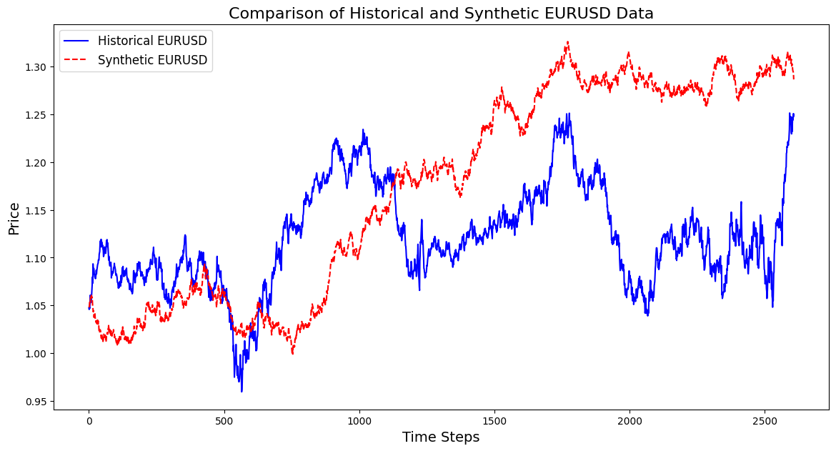
This visualization helps track how closely the synthetic data matches the real data, offering insights into the GAN's progress and highlighting areas for potential improvement during training.

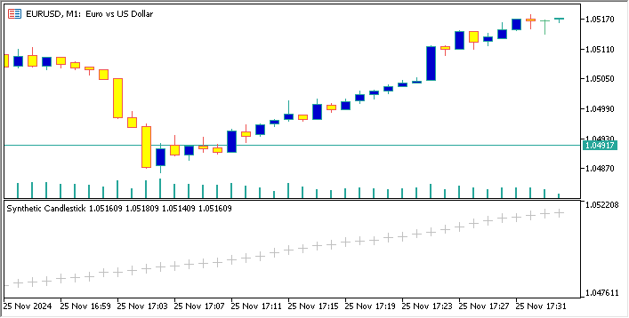
Below is a code that creates a synthetic currency pair based on EURUSD, and displays its candlesticks chart on the  EURUSD chart

//+------------------------------------------------------------------+
//|                                         Sythetic EURUSDChart.mq5 |
//|                                  Copyright 2024, MetaQuotes Ltd. |
//|                                             https://www.mql5.com |
//+------------------------------------------------------------------+
#property copyright "Copyright 2024, MetaQuotes Ltd."
#property link      "https://www.mql5.com"
#property version   "1.00"
#property indicator_separate_window  // Display in a seperate window
#property indicator_buffers 4        //Buffers for Open, High,Low,Close
#property indicator_plots 1           //Plot a single series(candlesticks)
//+------------------------------------------------------------------+
//| Indicator to generate and display synthetic currency data        |
//+------------------------------------------------------------------+

double openBuffer[];
double highBuffer[];
double lowBuffer[];
double closeBuffer[];

//+------------------------------------------------------------------+
//| Custom indicator initialization function                         |
//+------------------------------------------------------------------+
int OnInit()
  {
//---Set buffers for synthetic data
   SetIndexBuffer(0, openBuffer);
   SetIndexBuffer(1, highBuffer);
   SetIndexBuffer(2, lowBuffer);
   SetIndexBuffer(3, closeBuffer);
//---Define the plots for candle sticks
IndicatorSetString(INDICATOR_SHORTNAME, "Synthetic Candlestick");

//---Set the plot type for the candlesticks
   PlotIndexSetInteger(0, PLOT_DRAW_TYPE, DRAW_CANDLES);
   
   //---Setcolours for the candlesticks
   PlotIndexSetInteger(0, PLOT_COLOR_INDEXES, clrGreen);
   PlotIndexSetInteger(1, PLOT_COLOR_INDEXES, clrRed);
   //---Set the width of the candlesticks
   PlotIndexSetInteger(0, PLOT_LINE_WIDTH, 2);
//---Set up the data series(buffers as series arrays)
   ArraySetAsSeries(openBuffer, true);
   ArraySetAsSeries(highBuffer, true);
   ArraySetAsSeries(lowBuffer, true);
   ArraySetAsSeries(closeBuffer, true);

   return(INIT_SUCCEEDED);
  }
//+------------------------------------------------------------------+
//| Custom indicator iteration function                              |
//+------------------------------------------------------------------+
int OnCalculate(const int rates_total,
                const int prev_calculated,
                const datetime &time[],
                const double &open[],
                const double &high[],
                const double &low[],
                const double &close[],
                const long &tick_volume[],
                const long &volume[],
                const int &spread[])
  {
//---
   int start = MathMax(prev_calculated-1, 0);  //start from the most recent data
   double price =close[rates_total-1]; // starting price
   MathSrand(GetTickCount()); //initialize random seed
//---Generate synthetic data for thechart
   for(int i = start; i < rates_total; i++)
     {
      double change = (MathRand()/ 32768.0)* 0.0002 - 0.0002; //Random price change
      price += change ;    // Update price with the random change
      openBuffer[i]= price;
      highBuffer[i]= price + 0.0002;  //simulated high
      lowBuffer[i]= price - 0.0002; //simulated low
      closeBuffer[i]= price;

     }
//--- return value of prev_calculated for next call
   return(rates_total);
  }
//+------------------------------------------------------------------+

Analysis of Popular Metrics for Assessing GANs in Financial Modeling

Evaluating Generative Adversarial Networks (GANs) is crucial for determining whether their synthetic data accurately replicates real financial data. Here are key metrics used for assessment:

1. Mean Squared Error (MSE)

MSE measures the average squared difference between real and synthetic data points. A lower MSE indicates that the synthetic data closely resembles the real dataset, making it suitable for tasks like price prediction or portfolio management. Traders can use MSE to validate whether GAN-generated data reflects actual market movements.For example, a trader using a Generative Adversarial Network (GAN) to generate fake stock price data can measure entropy vs. utilizing the actual prices recorded in history to compute the Mean Squared Error (MSE). A low MSE proves the solidity of synthesized data as they match real market movements allowing using them for training AI models for predicting future price interactions.

2. Fréchet Inception Distance (FID)

Although commonly used in image generation, FID can also apply to financial data. It compares real and synthetic data distributions in feature space. A lower FID score implies better alignment between synthetic and real data, supporting applications like portfolio stress testing and risk estimation. For example, it manages a portfolio by helping compare synthetic distributions of returns with actual market returns. Hypothesis 3 indicates that since a lower FID score means that GAN-generated returns are closer mimics of actual return distributions, this shows that the GAN model is well suited for the performance of portfolio stress tests and risk estimation.

3. Kullback-Leibler (KL) Divergence

KL Divergence assesses how closely the synthetic data's probability distribution matches the real data's distribution. In finance, a low KL Divergence suggests that GAN-generated data captures critical properties like volatility clustering, making it effective for risk modeling and algorithmic trading. For example, models assess the generative model or GAN’s ability to recognize actual asset return distribution, in terms of tail risks and volatility clustering. A low KL Divergence means that the synthetic data has important features of realistic return risks, thus it is effective to apply risk models based on GAN data.

4. Discriminator Accuracy

The Discriminator measures how well it can differentiate between real and synthetic data. Ideally, as training progresses, the Discriminator's accuracy should approach 50%, indicating that the synthetic data is indistinguishable from real data. This validates the quality of GAN outputs for backtesting and future scenario modeling. For example, when used in algorithmic trading strategy helps in the flow validation process. Through observing this accuracy, traders will be well-positioned to see whether or not the GAN is creating realistic synthetic futures. High-quality and indistinguishable scenario matches the backtested data result from an accuracy hovering around 50%.

These metrics provide a comprehensive framework for evaluating GANs in financial modeling. They help developers improve synthetic data quality and ensure its applicability in tasks like portfolio management, risk assessment, and trading strategy validation.

Conclusion

Generative Adversarial Networks (GANs) allow traders and financial analysts to generate synthetic data, beneficial when real data is limited, costly, or sensitive. GANs provide reliable data for financial modeling, enhancing cash flow analysis in trading models. With foundational knowledge of GANs, traders can explore synthetic data generation independently to strengthen their analytical capabilities.

Future topics will cover advanced techniques like Wasserstein GANs and Progressive Growing for improved GAN stability and application in finance.

All code referenced in the article is attached below. The following table describes all the source code files that accompany the article.

File Name	Description
GAN_training_code.py	File training code for training the GAN
GAN_Inspired basic structure.mq5	File containing code for the GAN structure in MQL5
GAN_Model_building.py	File containing code for GAN structure in Python
MA Crossover GAN integrated.mq5	File containing the code for Expert Advisor tested on real and fake data
EURUSD_historical_synthetic_ comparison.py	File containing the code of comparison between historical and synthetic EURUSD
Synthetic EURUSDchart.mq5	File containing the code for creating synthetic chart on EURUSD chart
EURUSD_CSV.csv	File containing the synthetic data that is imported to test the expert advisor