Overcoming The Limitation of Machine Learning (Part 2): Lack of Reproducibility

I often receive encouraging feedback from our readers, but a recurring theme in private messages and comments is the difficulty some encounter when trying to replicate the results presented in our articles. Initially, this puzzled me, but after some reflection, a likely explanation emerged.

The global financial market operates as a massive and decentralized network. There are many brokers in the world, with new ones being registered daily, yet there is no single international authority to regulate these brokers or coordinate their price feeds. Each broker is free to source prices from their preferred proprietary feeds or data services, such as Reuters. 

Consequently, if you compare the EURUSD performance across two brokers-let’s call them Broker A and Broker B, you may find the same pair moving in opposite directions at the same moment. For instance, Broker A might report the EURUSD appreciating by 0.12% in a day, while Broker B records a depreciation of -0.65% for that same day.

The Heart of The Issue: Data Discrepancy Between Brokers

For this discussion, I randomly selected two brokers I, personally, use for independent trading. In line with our community guidelines, which prohibit broker promotion, their names have been redacted and replaced with “Broker A” and “Broker B.”

Using the MetaTrader 5 Python library, I requested four years of daily historical EURUSD data from both brokers. Upon review, I noticed that the timestamps didn’t align: one broker’s data extended back to September 2019, while the other’s only reached August 2020. Nevertheless, both returned exactly 1,460 rows of daily data, correctly fulfilling our request.

Given the decentralized nature of brokers, it’s expected that their operating time zones may differ. Less obvious, however, are the effects of daylight saving time, recognized public holidays, and other subtle discrepancies, all of which can further skew timestamp alignment.

We then calculated the 10-Day EURUSD return on both brokers and found that the numerical properties of the EURUSD symbol were inconsistent with each other. The average 10-Day EURUSD return with Broker A was 0.000267 while with Broker B, the average 10-Day return was -0.000352. This represents a difference of about 232% in the expected return of the same underlying asset.

To make matters worse, it appears that the expected returns from Broker A carry 21% more risk than the expected returns from Broker B. This was suggested to us by the fact that the variance in returns between Brokers grew by the same amount, 21%. 

Beginner's Note: The reader is intended to grasp that variance in returns is considered financial risk. Any introductory textbook on financial portfolio theory can demonstrate this to readers who may not have been aware of this principle beforehand.

In statistics, we can inquire whether 2 variables move in unison or if they move independently of each other by measuring their levels of correlation. Standardized correlation measures run from 1 to -1. A score of 1 implies that the variables move perfectly in the same directions, while a score of -1 implies the variables move perfectly in opposite directions. When we compared the coefficients of Pearson's Correlation metric between the 2 brokers, I, the writer, was honestly expecting correlation coefficients close to 1. However, the data demonstrated correlation levels of only 0.41. 

This suggests that any beliefs that the price levels of the EURUSD symbol will move in harmony across different brokers appears to be mathematically unfounded. Rather, the results of our test suggest that more than half of the time, the EURUSD market moves in different directions across different brokers.

Other important numerical qualities of the 2 brokers' quotes only reinforced the depths of the problems this article is bringing to the reader's attention. In our previous discussion on the limitations of AI, we showed the reader some of the pitfalls associated with metrics commonly used to build regression models, such as RMSE. The reader can find that article linked, here.

Briefly, we advised the reader to refrain from reading RMSE as a standalone metric, but rather to interpret this metric with a pinch of salt, by comparing the ratio of the performance of the model you intend to use (Residual Sum of Squares, RSS), against the error produced by a simple model that always predicts the average market return (Total Sum of Squares, TSS). The point was that readers may be surprised how challenging it may be to outperform the simpler model. The ratio of the RSS divided by the TSS informs us how efficiently we are outperforming the simple model.

One would expect that for the same symbol, this ratio ought to remain almost constant, even across different brokers. However, our ability to outperform a model predicting the average market return improved by 7% simply by changing brokers. This implies that the 10-Day EURUSD return is approximately 7% easier to forecast directly with Broker B, than it is with Broker A!

Statisticians often compare a distribution’s center to its standard deviation to learn more about the characteristics of a given distribution's tail. When this operation is reinterpreted to be applied to the 10-day EURUSD returns, we would learn a numerical method to compare which broker tends to produce outsized returns. By this line of reasoning, Broker B's 10-Day EURUSD returns appeared inflated by 147%.

By now, the problem we are facing should be clear: important numerical characteristics of the same symbol are not guaranteed to be consistent across brokers. As a result, the profitability of any given trading strategy cannot always be reliably reproduced between brokers.

Trading strategies that integrate AI models built using the ONNX API, or even natively in MQL5, may consistently fail to meet investor expectations, unless the additional time required to uniquely tailor AI to the intended broker becomes widely adopted practice. While this is time-consuming work, it is clearly critical work.

As you read this article, we will step-by-step recreate the production cycle most MQL5 developers may be following. We aim to use this article to illustrate that when a developer builds and optimizes their application using their private broker, in our case Broker B, but their client deploys that application with a different broker, Broker A, then trouble is not that far removed from the developer and his customer. Any developer following such a production cycle will most likely be left with mixed reviews on their products.

To avoid such unsatisfactory performance levels, MQL5 developers that wish to deliver reliable services may need to realize that their customers may be best served by having strategies and applications tailored to specific brokers for the safety of the consumers we wish to serve in the Marketplace.

Getting Started

We first need to import our standard numerical libraries.

#Load our libraries
import pandas as pd
import numpy as np
import matplotlib.pyplot as plt
import seaborn as sns
import MetaTrader5 as mt5

Define which time-frame and currency pair we will be focused on, and also how many rows of data we need.

#Let us define certain constants
TF = mt5.TIMEFRAME_D1
DATA = (365 * 4)
START = 1
PAIR = "EURUSD"

Start up your terminal.

#Log in to the terminal
if mt5.initialize():
   print('Logged in successfully')

else:
   print('Failed To Log In')

Logged in successfully

Let us analyze the difficulty of forecasting the EURUSD with broker A.

EURUSD_BROKER_A = pd.DataFrame(mt5.copy_rates_from_pos(PAIR,TF,START,DATA))
#Store the data we retrieved from broker A
EURUSD_BROKER_A.to_csv("EURUSD BROKER A.csv")

Now we shall repeat the same procedure for broker B.

#I have manually changed brokers using the MT5 terminal, you should also do the same on your side
EURUSD_BROKER_B = pd.DataFrame(mt5.copy_rates_from_pos(PAIR,TF,START,DATA))
#Store the data we retrieved from broker B
EURUSD_BROKER_B.to_csv("EURUSD BROKER B.csv")

Great! Now we have collected EURUSD historical data from both brokers, let us start looking into the empirical properties of these datasets, to see if the EURUSD Symbol is consistent across different brokers. We need to define how far into the future we shall be forecasting.

#Our forecasting horizon
HORIZON = 10

Read in both datasets.

EURUSD_BROKER_A = pd.read_csv("EURUSD BROKER A.csv")
EURUSD_BROKER_B = pd.read_csv("EURUSD BROKER B.csv")

The datasets have their time column currently being recorded in seconds, we would rather have human-readable time columns in date-month-year format. Let us build a method to do so.

def format_data(f_data):
    #First make a copy of the data, so we always preserve the original data
    f_data_copy = f_data.copy()
    #Format the time correctly, form seconds to human readable formats
    f_data_copy['time'] = pd.to_datetime(f_data_copy['time'],unit='s')
    return(f_data_copy)

Format our datasets.

A = format_data(EURUSD_BROKER_A)
B = format_data(EURUSD_BROKER_B)

Rename all columns accordingly, so that each column's name is suffixed by the letter of the broker that provided us with the data. All columns from Broker A or B will end with an A or B respectively. Let us now carefully examine the historical EURUSD data we have received from both brokers. Pay attention to the fact that both sets, have exactly 1 460 rows of Daily data, meaning that each broker correctly returned exactly 4 years Daily of data. What other differences can the reader observe? Have you taken a look at the tick volume?

# Rename all columns (except the join key)
B = B.rename(columns=lambda col: col + ' B' if col != 'id' else col)
A = A.rename(columns=lambda col: col + ' A' if col != 'id' else col)

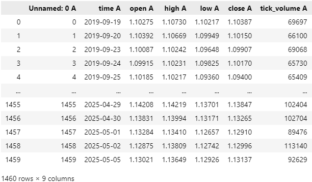
Fig. 1: The historical Daily EURUSD data we received from Broker A, with time-stamps as old as September 2019

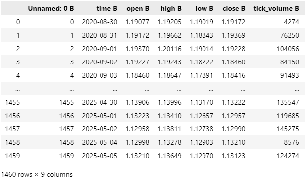
Fig. 2: The historical Daily EURUSD data we received from Broker B does not align with the time-stamps in Fig 1, but both are exactly 4 years

Let us now join the 2 datasets.

combined = pd.concat([A,B],axis=1)

Create a column full of just 0.

combined['Null'] = 0

Define the inputs.

inputs = ['open A','high A','low A','close A','tick_volume A','spread A','open B','high B','low B','close B','tick_volume B','spread B']

Calculate the 10-Day EURUSD return.

#Label the data
combined['A Target'] = combined['close A'].shift(-HORIZON) - combined['close A']
combined['B Target'] = combined['close B'].shift(-HORIZON) - combined['close B']

#Drop the last HORIZON rows of data
combined = combined.iloc[:-HORIZON,:]

The tick volume informs us how many price changes we have observed periodically. Periods of intense trading, will be given away by high tick volume, indicating that there was a lot of market activity and the opposite implies that the market was relatively quiet with little activity. Broker A appears to have a long-term uptrend in their tick volume data, suggesting that the open interest investors are showing appears to be growing over time. There are occasional large spikes in the plot, which may correspond to particularly busy periods whereby open interest in the EURUSD approaches a maximum.

plt.title('Broker A Daily EURUSD Tick Volume')
plt.plot(combined['tick_volume A'],color='black')
plt.ylabel('Tick Volume')
plt.xlabel('Historical Day')
plt.grid()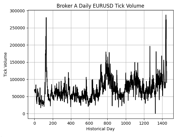

Fig. 3: The EURUSD tick volume we received from Broker A

When we compare the tick volume presented to us by Broker B in Fig. 4, against Fig. 3, we can clearly see large differences in reported activity levels. Broker B has almost no trend in their tick volume, when compared against Broker A. Fig. 4 is dense, with random spikes that do not appear as periodical as the spikes we observed in Fig. 3. 

plt.title('Broker B Daily EURUSD Tick Volume')
plt.plot(combined['tick_volume B'],color='black')
plt.ylabel('Tick Volume')
plt.xlabel('Historical Day')
plt.grid()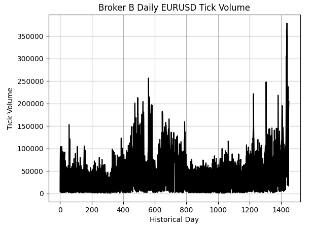

Fig. 4: The Daily EURUSD tick volume we received from Broker B

When we consider the average return and investor could expect when holding the EURUSD with each broker, we learn that both brokers offer different variations of the same symbol. Otherwise, if these 2 brokers were offering us identical versions of the same symbol, then shouldn't we have matching levels of expected return?

#What's the average 10-Day EURUSD return from both brokers
delta_return = str(((combined.iloc[:,-2:].mean()[0]-combined.iloc[:,-2:].mean()[1]) / combined.iloc[:,-2:].mean()[0]) * 100)

t = 'The Expected 10-Day EURUSD Return Differes by ' + delta_return[:5] + '% Between Our Brokers'

sns.barplot(combined.iloc[:,-2:].mean(),color='black')
plt.axhline(0,color='grey',linestyle='--')
plt.title(t)
plt.ylabel('Return')

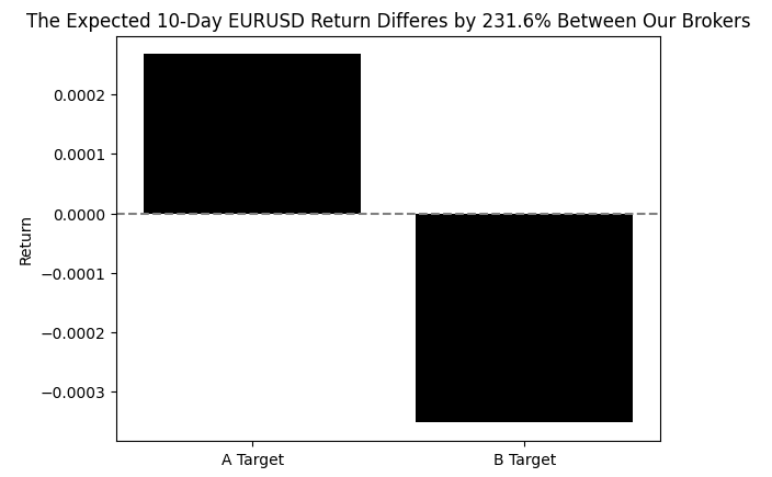
Fig. 5: The average market return between brokers lies on opposite sides of 0

Let us plot the returns generated by the 2 markets on top of each other. I will scale each of the returns so that both lines are centered at 0, and the displacement from 0 represents how many standard deviations we deviated from the average market return. We can right away see that there are many moments when the two lines are on opposite sides of the 0 line, and yet there are other times when the two lines follow each other. Recall that, casually speaking, we tend to assume these 2 lines are always following each other, but Fig. 6 shows us this is only true some of the time.

plt.plot(((combined.iloc[:,-1]-combined.iloc[:,-1].mean())/combined.iloc[:,-1].std()),color='red')
plt.plot(((combined.iloc[:,-2]-combined.iloc[:,-2].mean())/combined.iloc[:,-2].std()),color='black')
plt.grid()
plt.axhline(0,color='black',linestyle='--')
plt.ylabel('Std. Deviations From Expected 10-Day EURUSD Return')
plt.xlabel('Historical Days')
plt.title('EURUSD Returns from Different Brokers May Not Always Allign')
plt.legend(['Broker A','Broker B'])

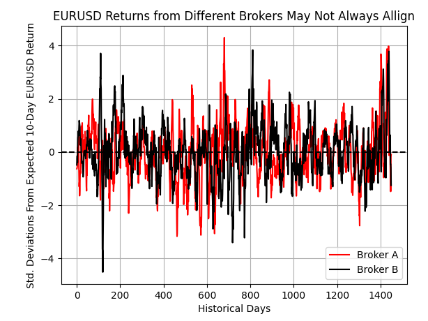
Fig. 6: Visualizing the 10-Day EURUSD returns being generated by 2 different brokers

Comparing the amount of variance in the returns offered by the brokers allows us to assess which broker is riskier, and which broker is offering us returns that are more certain. By this measure, Broker A's version of the EURUSD carries more risk associated with its returns when compared against Broker B.

#The variance of returns is not the same across both brokers, broker A is riskier
delta_var = str(((combined.iloc[:,-2:].var()[0]-combined.iloc[:,-2:].var()[1]) / combined.iloc[:,-2:].var()[0]) * 100)

t = 'Broker A EURUSD Returns Appear to Carry '+ delta_var[:5]+'% Additional Risk.'

sns.barplot(combined.iloc[:,-2:].var(),color='black')
plt.axhline(np.min(combined.iloc[:,-2:].var()),color='red',linestyle=':')
plt.title(t)
plt.ylabel('Vriance of Returns')

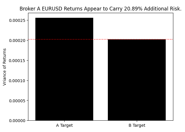
Fig. 7: Broker A's returns carry 21% more risk than Broker B's returns, at this point, do you still consider these Symbols to be "the same"?

When we turn our attention to considering the largest drawdown recorded by both brokers, we still fail to solicit coherent observations. The largest drawdown demonstrated by both markets differed by about 37% between our 2 brokers. All this appears to suggest that Broker B is intelligently cushioning their clients from the volatility of the EURUSD market by offering a truncated perspective of the foreign exchange market.

#Broker A also demonstrated the largest drawdown ever in our 4 year sample window
delta = (((combined.iloc[:,-2:].min()[0]-combined.iloc[:,-2:].min()[1]) / combined.iloc[:,-2:].min()[0]) *100)
delta_s = str(delta)

t = 'The Largest Negative 10-Day EURUSD Return Grew By: ' + delta_s[:5] + ' %'

sns.barplot(combined.iloc[:,-2:].min(),color='black')
plt.axhline(np.max(combined.iloc[:,-2:].min()),color='red',linestyle=':')
plt.title(t)
plt.ylabel('Return')

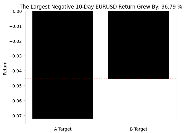
Fig. 8: Broker A demonstrated the largest drawdown in returns by 36.79%, well ahead of the largest drawdown from Broker B

Overlaying the distribution of the 10-Day EURUSD return generated by both brokers shows that both Brokers truly are not offering the same view of the market. As we explained in the introduction of our discussion, each broker is free to acquire their price feeds from whichever source they pick. This decentralized pricing scheme, means that each broker may be offering arbitrarily different perspectives on any particular market.

sns.histplot(((combined.iloc[:,-2]-combined.iloc[:,-2].mean())/combined.iloc[:,-2].std()),color='black')
sns.histplot(((combined.iloc[:,-1]-combined.iloc[:,-1].mean())/combined.iloc[:,-1].std()),color='red')
plt.xlabel('Std. Deviations From The Expected Return')
plt.ylabel('Frequency')
plt.title('Comparing The Distribution of 10-Day EURUSD Returns Between 2 Brokers')
plt.grid()
plt.legend(['Broker A','Broker B'])

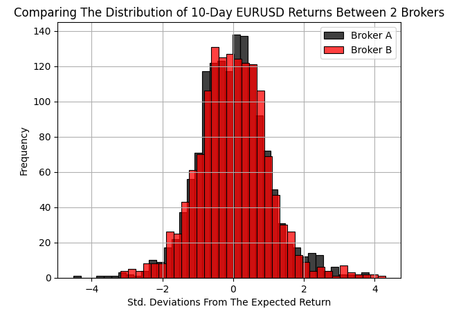
Fig. 9: Comparing the distribution of returns generated by the 2 markets

Additionally, when we analyze the correlation levels between brokers, we find that the market prices are poorly correlated with each other. Meaning, as we said earlier, more than half of the time, price levels between these 2 particular brokers could be evolving in opposite directions.

sns.heatmap(combined.loc[:,inputs].corr(),annot=True)

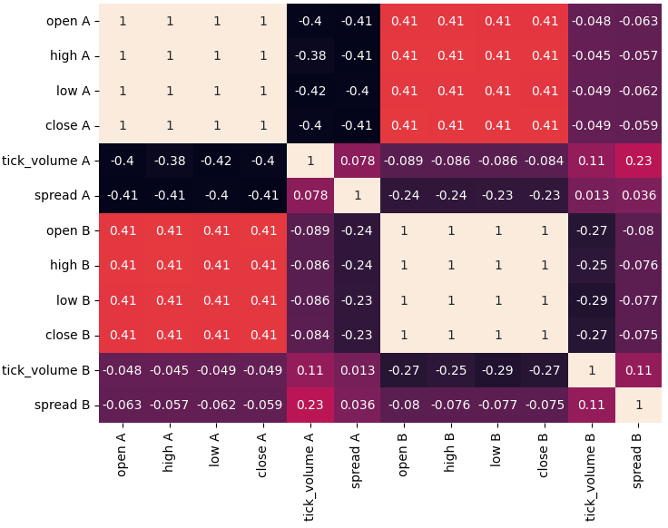
Fig. 10: Visualizing the correlation levels shows us that both broker's symbols move almost independently the majority of the time

Let us now see if our predictive abilities remain consistent across brokers.

from sklearn.model_selection import train_test_split,TimeSeriesSplit,cross_val_score
from sklearn.linear_model import Ridge

Create a time series validation object.

tscv = TimeSeriesSplit(n_splits=5,gap=HORIZON)

Write a method that will return us a new model to use.

def get_model():
    return(Ridge())

Split the data, and be sure not to shuffle it.

train , test = train_test_split(combined,shuffle=False,test_size=0.5)

Record our error levels when using the column we purposefully filled with just 0's. This will force the model to always predict the average value of the target. Recall that when all inputs are 0, a linear model will predict the intercept. Or simply put, this model informs us how well we can perform in this market if we always predict the average market return. Failing to beat this model informs us that we have no skill.

This benchmark is called the TSS. We defined the TSS in the introduction of our discussion. Our goal here is to measure the TSS across both brokers, and then see compare our ability to outperform this benchmark across brokers.

broker_a_tss = np.mean(np.abs(cross_val_score(get_model(),train.loc[:,['Null']],train.loc[:,'A Target'],scoring='neg_mean_squared_error',n_jobs=-1,cv=tscv)))
broker_a_rss = np.mean(np.abs(cross_val_score(get_model(),train.loc[:,inputs[0:(len(inputs)//2)]],train.loc[:,'A Target'],scoring='neg_mean_squared_error',n_jobs=-1,cv=tscv)))

broker_b_tss = np.mean(np.abs(cross_val_score(get_model(),train.loc[:,['Null']],train.loc[:,'B Target'],scoring='neg_mean_squared_error',n_jobs=-1,cv=tscv)))
broker_b_rss = np.mean(np.abs(cross_val_score(get_model(),train.loc[:,inputs[(len(inputs)//2):]],train.loc[:,'B Target'],scoring='neg_mean_squared_error',n_jobs=-1,cv=tscv)))

Surprisingly, it is easier for us to outperform the TSS on Broker B than it is with Broker A! This means the future 10-Day EURUSD return is not always efficient as we move from broker to broker.

res = [(broker_a_rss/broker_a_tss),(broker_b_rss/broker_b_tss)]

eff = str(((res[0] - res[1])/res[1]) * 100)

t = 'The EURUSD Appears ' + eff[0:4] + '% Easier To Forecast With Broker B'

sns.barplot(res,color='black')
plt.axhline(np.min(res),color='red',linestyle=':')
plt.ylabel('5-Fold Cross Valiated Ratio of RSS/TSS ')
plt.title(t)
plt.xticks([0,1],['Broker A','Broker B'])

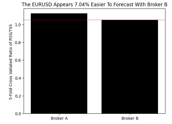
Fig. 11: The 10-Day future EURUSD return is easier to forecast on using Broker B

Since we have established which broker we want to focus on, select the input data we received from Broker B.

b_inputs = inputs[len(inputs)//2:]

Now let us build a new model altogether.

from sklearn.ensemble import GradientBoostingRegressor

model = GradientBoostingRegressor()

Fit the model on all the data we have from Broker B.

model.fit(train.loc[:,b_inputs[:-2]],train['B Target'])

Now let us get ready to export our model to ONNX format so that we can easily integrate our AI model into our MQL5 application.

import skl2onnx,onnx

Define the number of inputs our ONNX model accepts.

initial_types = [('float_input',skl2onnx.common.data_types.FloatTensorType([1,4]))]

Convert the ONNX model into an ONNX prototype.

onnx_proto = skl2onnx.convert_sklearn(model,initial_types=initial_types,target_opset=12)

Save the ONNX prototype to disk.

onnx.save(onnx_proto,"EURUSD GBR D1.onnx")

Getting Started in MQL5

Now that we have our ONNX model ready, we can begin building our MQL5 application. First, load the libraries we need.

//+------------------------------------------------------------------+
//|                                                       EURUSD.mq5 |
//|                                               Gamuchirai Ndawana |
//|                    https://www.mql5.com/en/users/gamuchiraindawa |
//+------------------------------------------------------------------+
#property copyright "Gamuchirai Ndawana"
#property link      "https://www.mql5.com/en/users/gamuchiraindawa"
#property version   "1.00"

//+------------------------------------------------------------------+
//| System Constants Definitions                                     |
//+------------------------------------------------------------------+
#include  <Trade\Trade.mqh>
CTrade Trade;

We will also need system constants to ensure that our application reflects the important parameters we defined earlier in our discussion, such as the 10-Day return period.

//+------------------------------------------------------------------+
//| System Constants Definitions                                     |
//+------------------------------------------------------------------+
#define  ONNX_INPUT_SHAPE 4
#define  ONNX_OUTPUT_SHAPE 1
#define  SYSTEM_TIME_FRAME PERIOD_D1
#define  RETURN_PERIOD 10
#define  TRADING_VOLUME SymbolInfoDouble(Symbol(),SYMBOL_VOLUME_MIN)

Load the ONNX file as a system resource so that it is compiled with our application.

//+------------------------------------------------------------------+
//| System Resources                                                 |
//+------------------------------------------------------------------+
#resource "\\Files\\Broker Manipulation\\EURUSD GBR D1.onnx" as const uchar onnx_proto[];

A few global variables will be necessary for us to implement our trading strategy.

//+------------------------------------------------------------------+
//| Global Variables                                                 |
//+------------------------------------------------------------------+
long   model;
int    position_timer;
double bid,ask;
double o,h,l,c;
bool   bullish;
double sl_width;

When our system is initialized for the first time, we will set up our ONNX model and then reset important global variables for our trading strategy.

//+------------------------------------------------------------------+
//| Expert initialization function                                   |
//+------------------------------------------------------------------+
int OnInit()
  {
//---
   model = OnnxCreateFromBuffer(onnx_proto,ONNX_DATA_TYPE_FLOAT);

   ulong input_shape[] = {1,ONNX_INPUT_SHAPE};
   ulong output_shape[] = {1,ONNX_OUTPUT_SHAPE};

   if(model == INVALID_HANDLE)
     {
      Comment("Failed To Load EURUSD Auto-Encoder-Decoder: ",GetLastError());
      return(INIT_FAILED);
     }

   if(!OnnxSetInputShape(model,0,input_shape))
     {
      Comment("Failed To Set EURUSD Auto-Encoder-Decoder Input Shape: ",GetLastError());
      return(INIT_FAILED);
     }

   else
      if(!OnnxSetOutputShape(model,0,output_shape))
        {
         Comment("Failed To Set EURUSD Auto-Encoder-Decoder Output Shape: ",GetLastError());
         return(INIT_FAILED);
        }

   position_timer = 0;
   sl_width = 30;
//---
   return(INIT_SUCCEEDED);
  }

If we are no longer using our trading strategy, free up the resources that were being consumed by our ONNX model.

//+------------------------------------------------------------------+
//| Expert deinitialization function                                 |
//+------------------------------------------------------------------+
void OnDeinit(const int reason)
  {
//---
   OnnxRelease(model);
  }

Whenever we receive updated prices, store the new price levels once a day and then if we have no open positions, we will obtain a forecast from our model and then trade accordingly. Otherwise, if we already have an open trade, then we will try and trail our stop-loss if possible whilst we count down our 10-Day holding period for each trade.

//+------------------------------------------------------------------+
//| Expert tick function                                             |
//+------------------------------------------------------------------+
void OnTick()
  {
//---
   static datetime time_stamp;
   datetime current_time = iTime(Symbol(),SYSTEM_TIME_FRAME,0);

   if(time_stamp != current_time)
     {
      time_stamp = current_time;
      ask = SymbolInfoDouble(Symbol(),SYMBOL_ASK);
      bid = SymbolInfoDouble(Symbol(),SYMBOL_BID);
      o = iOpen(Symbol(),SYSTEM_TIME_FRAME,1);
      h = iHigh(Symbol(),SYSTEM_TIME_FRAME,1);
      l = iLow(Symbol(),SYSTEM_TIME_FRAME,1);
      c = iClose(Symbol(),SYSTEM_TIME_FRAME,1);
      bullish = (o < c) && (c > iClose(Symbol(),SYSTEM_TIME_FRAME,2));

      if(PositionsTotal() == 0)
        {
         position_timer = 0;
         find_setup();
        }

      else
         if(PositionsTotal() > 0)
           {
            if(PositionSelect(Symbol()))
              {
               long position_type = PositionGetInteger(POSITION_TYPE);
               double current_sl = PositionGetDouble(POSITION_SL);
               double new_sl;

               //--- Buy Trades
               if(position_type == POSITION_TYPE_BUY)
                 {
                  new_sl = bid - ((h-l)*sl_width);
                  if(new_sl > current_sl)
                     Trade.PositionModify(Symbol(),new_sl,0);
                 }

               //--- Sell Trades
               else
                  if(position_type == POSITION_TYPE_SELL)
                    {
                     new_sl = ask + ((h-l)*sl_width);
                     if(new_sl < current_sl)
                        Trade.PositionModify(Symbol(),new_sl,0);
                    }
              }

            if(position_timer < RETURN_PERIOD)
               position_timer+=1;

            else
               Trade.PositionClose(Symbol());
           }
     }
  }

Finally, this function will obtain a forecast from our model, and then check if we have a valid trading opportunity.

//+------------------------------------------------------------------+
//| Find A Trading Setup                                             |
//+------------------------------------------------------------------+
void find_setup(void)
  {
   vectorf model_inputs(ONNX_INPUT_SHAPE);

   model_inputs[0] = (float) iOpen(Symbol(),SYSTEM_TIME_FRAME,0);
   model_inputs[1] = (float) iHigh(Symbol(),SYSTEM_TIME_FRAME,0);
   model_inputs[2] = (float) iLow(Symbol(),SYSTEM_TIME_FRAME,0);
   model_inputs[3] = (float) iClose(Symbol(),SYSTEM_TIME_FRAME,0);

   vectorf model_output(ONNX_OUTPUT_SHAPE);

   if(!OnnxRun(model,ONNX_DATA_TYPE_FLOAT,model_inputs,model_output))
     {
      Comment("Failed To Get A Prediction From Our Model: ",GetLastError());
      return;
     }

   else
     {
      Comment("Prediction: ",model_output[0]);

      vector open,close;

      open.CopyRates(Symbol(),SYSTEM_TIME_FRAME,COPY_RATES_OPEN,1,2);
      close.CopyRates(Symbol(),SYSTEM_TIME_FRAME,COPY_RATES_CLOSE,1,2);

      if(open.Mean() < close.Mean())
        {
         if((model_output[0] > 0) && (bullish))
            Trade.Buy(TRADING_VOLUME,Symbol(),ask,(bid - ((h-l) * sl_width)),0);
        }


      else
         if(open.Mean() > close.Mean())
           {
            if((model_output[0] < 0) && (!bullish))
               Trade.Sell(TRADING_VOLUME,Symbol(),bid,(ask + ((h-l) * sl_width)),0);
           }
     }
  }

Do not forget to undefine any system constants you create in your application.

//+------------------------------------------------------------------+
//| Undefine System Constants                                        |
//+------------------------------------------------------------------+
#undef  ONNX_INPUT_SHAPE
#undef  ONNX_OUTPUT_SHAPE
#undef  SYSTEM_TIME_FRAME
#undef  TRADING_VOLUME
#undef  RETURN_PERIOD
//+------------------------------------------------------------------+

The date periods we will use for our back-test are out-of-sample from our model training period. These dates will be held constant for both our tests on Broker A and Broker B. Recall that Broker B symbolizes the broker that an MQL5 developer uses to build their application, while Broker A symbolizes the broker his clients may end up deploying the application with.

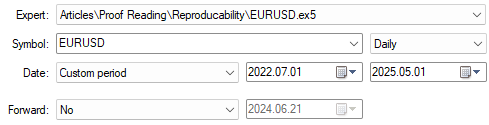
Fig. 12: Select the input dates for our test period

Both settings specified in Fig. 12 above and Fig. 13 below will be fixed across both tests we run.

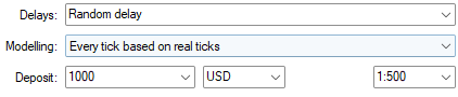
Fig. 13: We will also select challenging modelling settings to get a realistic expectation of our strategy's ability

As we can see in Fig. 14, our strategy appears promising when we test it with Broker B. It handles out-of-sample data well, and encourages us to spend more time refining the strategy to get the best performance out of it. However, the point we are trying to establish with the reader is that it may be naive to always think that improvements made with one broker, will correspond meaningfully with any other broker.

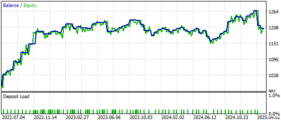
Fig. 14: The equity curve produced by our strategy has a positive trend when applied to the intended broker

However, after applying the same strategy with Broker A, we could no longer observe that positive uptrend in account balance that we observed with Broker B. The strategy clearly delivers very little value to us, if we change brokers, without changing the underlying model. Developers must understand that this is not always their fault. It is challenging for any developer to customize their models for every broker that exists under the sun.

However, this is a visual way to conceive the problem. Developers and their customers may be on entirely different pages, if their relationships are not defined carefully enough. 

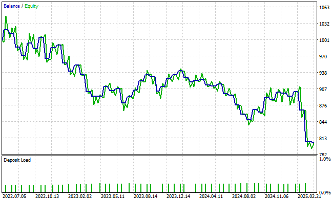
Fig. 15: When deploying our strategy with Broker A, we fail to reproduce the uptrend in account balance that we worked hard for

We can also take a closer look at a more detailed analysis of our performance with broker B in Fig. 16, and contrast this against how our model performed with broker A in Fig. 17. 

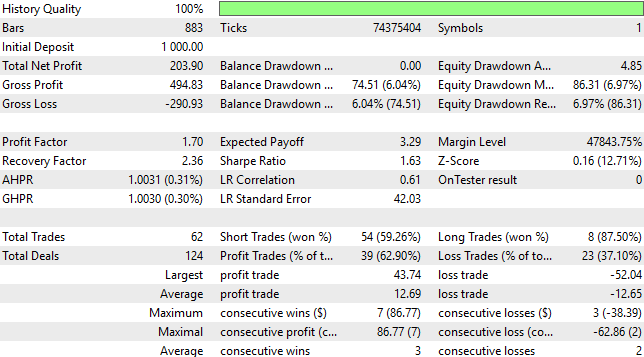
Fig. 16: A detailed analysis of our trading performance when we focus on the intended broker

We can clearly see that building a strategy that will perform meaningfully across multiple brokers is certainly not a trivial matter. As machine learning models become more complex, they also grow more sensitive to slight changes in their inputs. These variations in the numerical properties of the symbol can have devastating effects on our ability to share and meaningfully reproduce trading strategies. 

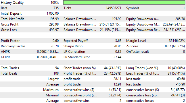
Fig. 17: A detailed analysis of the strategy trying to work on broker that it has not been trained with

Conclusion

The decentralized nature of global financial markets imposes real-world limitations that make it difficult for our community to reproduce each other’s findings. Brokers offer no guarantees that their prices will match, which means that inefficiencies you exploit with your broker may not exist with mine, even when using the same strategy on the same symbol.

Depending on your preferred role in our community, these insights have practical implications:

• If you enjoy using the “Freelance” section of the MQL5 website, specify your broker when requesting applications, and ask developers to create demo accounts with your broker to ensure you receive tailored solutions. Avoid making casual and broad requests such as "EURUSD Trading Application Wanted" because as we have seen, it may be safer for you to be as detailed as possible.
• Users that frequently purchase applications on the Marketplace now understand why broker-specific products can offer greater value than those claiming universal utility.
• Signal subscribers can maximize satisfaction by selectively choosing signal providers who use the same broker, ensuring reported and realized returns always align.
• Finally, my fellow MQL5 developers gain a clearer understanding of what it may take for us to deliver consistent products and reliable services that will keep our clients happy.

By recognizing these challenges, we can work towards more reproducible, broker-specific solutions that benefit everyone in our diverse and inclusive community. This article was designed to be an illustration of the dangers of associated with trying to share 1 ONNX model across different brokers. As MQL5 Developers, I believe we should hold ourselves accountable to higher standards of practice, and avoid exposing our customers to such dangers.

File Name	File Description
Requesting Broker Data.ipynb	The Jupyter Notebook we used to fetch historical Daily EURUSD data from our 2 brokers.
Analyzing Broker Data.ipynb	The Jupyter Notebook we used to test for consistency in the historical Daily EURUSD data from our 2 brokers.
EURUSD.mq5	The Expert Advisor we built to assess our profitability following the same model on 2 different brokers.