Gain an Edge Over Any Market (Part III): Visa Spending Index

Introduction

In the age of big data, there are almost infinite sources of alternative data available to the modern investor. Each data set holds the potential to yield higher accuracy levels when forecasting market returns. However, few data sets deliver on this promise. In this series of article, we will help you explore the vast landscape of alternative data, to assist you in making an informed decision whether you should include these data sets in your analysis, on the other hand, if these datasets render unsatisfactory results, then we may help save your time.

Our rationale is that, by considering alternative datasets not directly available in the MetaTrader 5 Terminal, we may uncover variables that predict price levels with relatively more accuracy in comparison with the casual market participant that relies solely on market quotes.

Synopsis of Trading Strategy

VISA is an American multinational payment services company. It was founded in 1958, and today the company operates one of the largest transactions processing networks in the world. VISA are well positioned to be a source of reputable alternative data because they have penetrated almost every market in the developed world. Furthermore, the Federal Reserve Bank of St. Louis also collect some of their macroeconomic data from VISA.

In this discussion, we’re going to analyze the VISA Spending Momentum Index (SMI). The Index is a macroeconomic indicator of consumer spending behavior. The data is aggregated by VISA, using their proprietary networks and branded VISA debit and credit cards. All the data is depersonalized and is mostly collected in the United States. As VISA continues to aggregate data from different markets, this index may eventually become a benchmark of global consumer behavior.

We will use an API service provided by the Federal Reserve Bank of St Louis to retrieve the VISA SMI datasets. The Federal Reserve Economic Database (FRED) API allows us to access hundreds of thousands of different economic time series data that have been collected from across the world.

Synopsis of the Methodology

The SMI data is released monthly by VISA, and contains less than 200 rows at the time of writing. Therefore, we need a modelling technique that is simultaneously resistant to over-fitting and flexible enough to capture complex relationships. This may be an ideal job for a neural network.

We optimized 5 parameters of a deep neural network to classify the changes in the EURUSD given a set of ordinary open, high, low and close price with 3 additions inputs, being the VISA datasets. Our optimized model was able to achieve 71% accuracy in validation, well, outperforming the default model. However, let the reader bear in mind this accuracy was on monthly data!

We employed 1000 iterations of a randomized search algorithm to optimize the deep neural network, and successfully trained the model without over-fitting to the training data. As impressive as these results may sound, we cannot confidently assert that the relationship observed is reliable. Our feature selection algorithms discarded all 3 VISA datasets when selecting the most important features in a non-parametric fashion. Furthermore, all 3 VISA data sets have relatively low mutual information scores, which may indicate to us the datasets may be independent or that we have failed to expose the relationship in a meaningful way for our model.

Data Extraction

To fetch the data we need, you must first create an account on the FRED website. After creating an account, you can use your FRED API key to access the economic time-series data held by the Federal Reserve of St. Louis and following along with our discussion. Our market data on EURUSD quotes will be fetched directly from the Terminal using the MetaTrader 5 Python API.

To get started, first load the libraries we need.

#Import the libraries we need
import pandas as pd
import seaborn as sns
import numpy as np
from fredapi import Fred
import MetaTrader5 as mt5
from datetime import datetime
import time
import pytz

Now set up your FRED API key and fetch the data we need.

#Let's setup our FredAPI
fred = Fred(api_key="ENTER YOUR API KEY")
visa_discretionary = pd.DataFrame(fred.get_series("VISASMIDSA"),columns=["visa d"])
visa_headline   = pd.DataFrame(fred.get_series("VISASMIHSA"),columns=["visa h"])
visa_non_discretionary = pd.DataFrame(fred.get_series("VISASMINSA"),columns=["visa nd"])

Define the forecast horizon.

#Define how far ahead we want to forecast
look_ahead = 10

Visualize the Data

Let us visualize all three datasets.

visa_discretionary.plot(title="VISA Spending Momentum Index: Discretionary")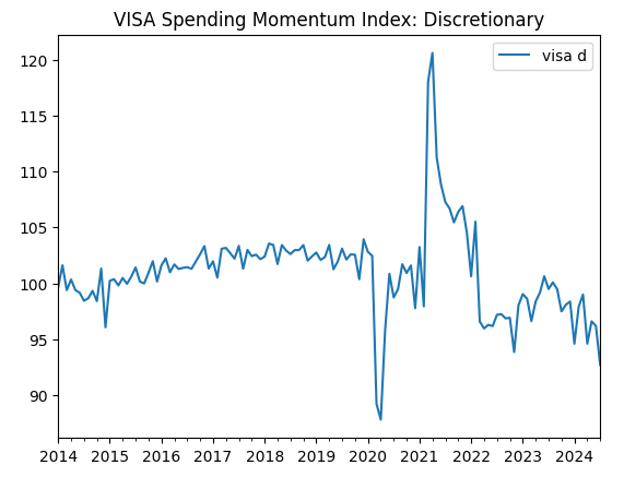

Fig 1: The first VISA Dataset

Now let us visualize the second dataset.

visa_headline.plot(title="VISA Spending Momentum Index: Headline")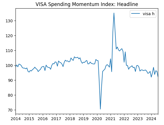

Fig 2: The second VISA dataset

And finally, our third VISA dataset.

visa_non_discretionary.plot(title="VISA Spending Momentum Index: Non-Discretionary")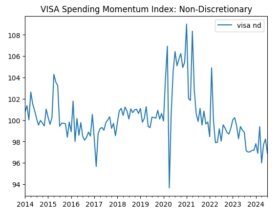

Fig 3: The third VISA dataset

The first two datasets appear almost identical, furthermore as we shall see later in our discussion, they have correlation levels of 0.89, meaning they may contain the same information. This suggests to us that we may drop one and keep the other. However, we will allow our feature selection algorithm to decide if that is necessary.

Fetching Data From Our MetaTrader 5 Terminal

We will now initialize our terminal.

#Initialize the terminal
mt5.initialize()

Now we shall specify our timezone.

#Set timezone to UTC
timezone = pytz.timezone("Etc/UTC")

Create a datetime object.

#Create a 'datetime' object in UTC
utc_from = datetime(2024,7,1,tzinfo=timezone)

Fetching the data from MetaTrader 5 and wrapping it in a pandas data frame.

#Fetch the data
eurusd = pd.DataFrame(mt5.copy_rates_from("EURUSD",mt5.TIMEFRAME_MN1,utc_from,visa_headline.shape[0]))

Let us label the data and use the timestamp as our index.

#Label the data
eurusd["target"] = np.nan
eurusd.loc[eurusd["close"] > eurusd["close"].shift(-look_ahead),"target"] = 0
eurusd.loc[eurusd["close"] < eurusd["close"].shift(-look_ahead),"target"] = 1
eurusd.dropna(inplace=True)
eurusd.set_index("time",inplace=True)

Now we shall merge the datasets using the dates they share.

#Let's merge the datasets
merged_data = eurusd.merge(visa_headline,right_index=True,left_index=True)
merged_data = merged_data.merge(visa_discretionary,right_index=True,left_index=True)
merged_data = merged_data.merge(visa_non_discretionary,right_index=True,left_index=True)

Exploratory Data Analysis

We are ready to explore our data. Scatter plots are helpful for visualizing the relationship between two variables. Let us observe the scatter plots created by each of the VISA datasets plotted against the closing price. The blue dots summarize the instances when price proceeded to fall over the next 10 candles, whilst the orange dots summarize the converse.

Although the separation is noisy towards the center of the plot, it appears that at the extreme levels the VISA datasets separate up and down moves reasonably well.

#Let's create scatter plots
sns.scatterplot(data=merged_data,y="close",x="visa h",hue="target").set(title="EURUSD Close Against VISA Momentum Index: Headline")

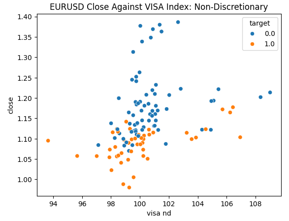
Fig 4: Plotting our Non-Discretionary VISA data set against the EURUSD close

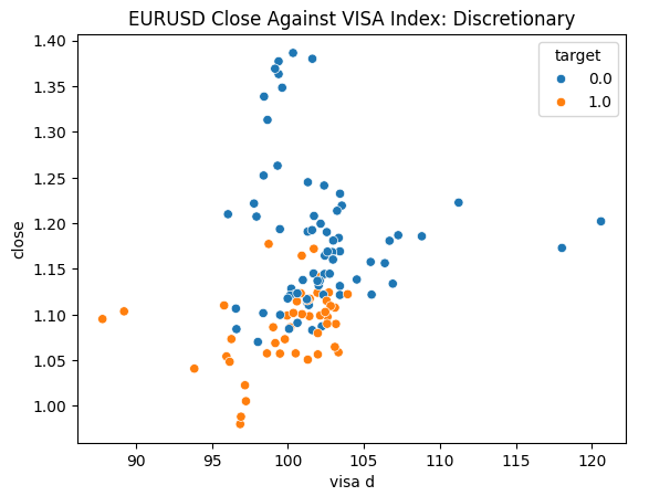
Fig 5: Plotting our Discretionary VISA data set against the EURUSD close

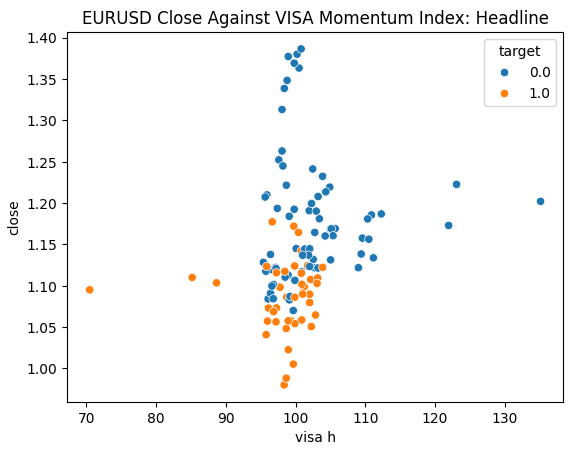
Fig 6: Plotting our Headline VISA data set against the EURUSD close

The correlation levels between the VISA datasets and the EURUSD market are moderate and all positive valued. None of the correlation levels are particularly interesting for our us. However, it is worth noting that the positive value indicates the two variables tend to rise and fall together. Which is inline with our understanding of macroeconomics, consumer expenditure in the USA has some level of influence on exchange rates. If consumers collectively chose not to spend, then their actions will reduce the total currency in circulation, which may cause the Dollar to appreciate.

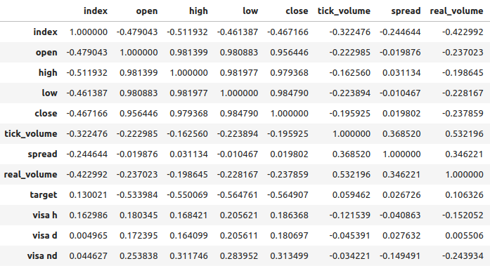
Fig 7: Correlation analysis of our dataset

Feature Selection

How important is the relationship between our target and our new features? Let us observe if the new features will be eliminated by our feature selection algorithm. If our algorithm does not select any of the new variables, then this may indicate that the relationship isn’t reliable.

The forward selection algorithm starts off with a null model and adds one feature at a time, from there it selects the best single variable model and then starts searching for a second variable and so on. It will return the best model it built to us. In our study, only the Open price was selected by the algorithm, indicating to us that the relationship may not be stable.

Import the libraries we need.

#Let's see which features are the most important
from mlxtend.feature_selection import SequentialFeatureSelector as SFS
from mlxtend.plotting import plot_sequential_feature_selection as plot_sfs
import matplotlib.pyplot as plt

Create the forward selection object.

#Create the forward selection object
sfs = SFS(
        MLPClassifier(hidden_layer_sizes=(20,10,4),shuffle=False,activation=tuner.best_params_["activation"],solver=tuner.best_params_["solver"],alpha=tuner.best_params_["alpha"],learning_rate=tuner.best_params_["learning_rate"],learning_rate_init=tuner.best_params_["learning_rate_init"]),
        k_features=(1,train_X.shape[1]),
        forward=False,
        scoring="accuracy",
        cv=5
).fit(train_X,train_y)

Let us plot the results.

fig1 = plot_sfs(sfs.get_metric_dict(),kind="std_dev")
plt.title("Neural Network Backward Feature Selection")
plt.grid()

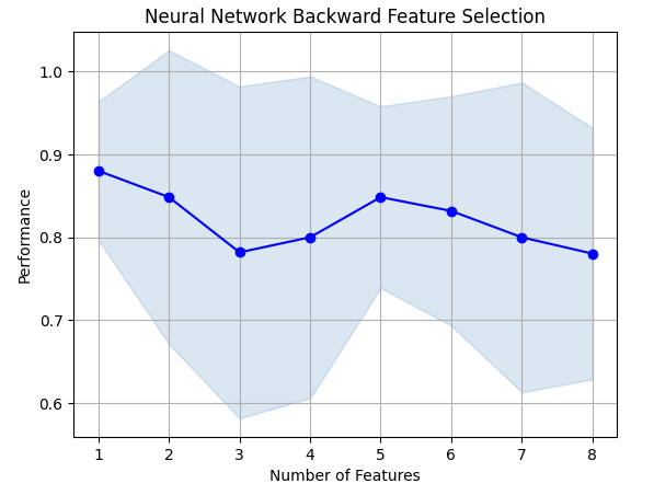
Fig 8: As we increased the number of features in the model, our performance got worse

Unfortunately, our accuracy kept falling as we added more features. This may either mean that the association simply isn't that strong, or we are not exposing the association in a way our model can interpret. So it appears a model with 1 feature may still be able to get the job done.

The best feature we identified.

sfs.k_feature_names_

('open',)

Let us now observe our mutual information (MI) scores. MI informs us how much potential each variable has to predict the target, MI scores are positive valued and range from 0 until infinity in theory, but in practice we rarely observe MI scores above 2 and an MI score above 1 is good.

Import the MI classifier from scikit-learn.

#Mutual information
from sklearn.feature_selection import mutual_info_classif

The MI score for the headline dataset.

#Mutual information from the headline visa dataset, 
print(f"VISA Headline dataset has a mutual info score of: {mutual_info_classif(train_X.loc[:,['visa h']],train_y)[0]}")

VISA Headline dataset has a mutual info score of: 0.06069528690724346

The MI score for the Discretionary dataset.

#Mutual information from the second visa dataset, 
print(f"VISA Discretionary dataset has a mutual info score of: {mutual_info_classif(train_X.loc[:,['visa d']],train_y)[0]}")

VISA Discretionary dataset has a mutual info score of: 0.1277119388376886

All our datasets had poor MI scores, this may be a compelling reason to try applying different transformations to the VISA dataset, and hopefully, we may uncover a stronger association.

Parameter Tuning

Let us now attempt to tune our deep neural network to forecast the EURUSD. Before that, we need to scale our data. First, reset the index of the merged dataset.

#Reset the index
merged_data.reset_index(inplace=True)

Define the target and the predictors.

#Define the target
target = "target"
ohlc_predictors = ["open","high","low","close","tick_volume"]
visa_predictors = ["visa d","visa h","visa nd"]
all_predictors = ohlc_predictors + visa_predictors

Now we shall scale and transform our data. From each value in our dataset, we will subtract the mean and divide by the standard deviation of that respective column. It is worth noting that this transformation is sensitive to outliers.

#Let's scale the data
scale_factors = pd.DataFrame(index=["mean","standard deviation"],columns=all_predictors)

for i in np.arange(0,len(all_predictors)):
        #Store the mean and standard deviation for each column
        scale_factors.iloc[0,i] = merged_data.loc[:,all_predictors[i]].mean()
        scale_factors.iloc[1,i] = merged_data.loc[:,all_predictors[i]].std()
        merged_data.loc[:,all_predictors[i]] = ((merged_data.loc[:,all_predictors[i]] - scale_factors.iloc[0,i]) / scale_factors.iloc[1,i])

scale_factors

Taking a look at the scaled data.

#Let's see the normalized data
merged_data

Importing standard libraries.

#Lets try to train a deep neural network to uncover relationships in the data
from sklearn.neural_network import MLPClassifier
from sklearn.model_selection import RandomizedSearchCV
from sklearn.model_selection import train_test_split
from sklearn.metrics import accuracy_score

Create a train-test split.

#Create train test partitions for our alternative data
train_X,test_X,train_y,test_y = train_test_split(merged_data.loc[:,all_predictors],merged_data.loc[:,"target"],test_size=0.5,shuffle=False)

Tuning the model to the available inputs. Recall that we must first pass the model we want to tune, and then specify the parameters of the model we are interested in. Afterward, we need to indicate how many folds we aim to use for cross validation.

tuner = RandomizedSearchCV(MLPClassifier(hidden_layer_sizes=(20,10,4),shuffle=False),
                        {
                                "activation": ["relu","identity","logistic","tanh"],
                                "solver": ["lbfgs","adam","sgd"],
                                "alpha": [0.1,0.01,0.001,(10.0 ** -4),(10.0 ** -5),(10.0 ** -6),(10.0 ** -7),(10.0 ** -8),(10.0 ** -9)],
                                "learning_rate": ["constant", "invscaling", "adaptive"],
                                "learning_rate_init": [0.1,0.01,0.001,(10.0 ** -4),(10.0 ** -5),(10.0 ** -6),(10.0 ** -7),(10.0 ** -8),(10.0 ** -9)],
                        },
                        cv=5,
                        n_iter=1000,
                        scoring="accuracy",
                        return_train_score=False
                        )

Fitting the tuner.

tuner.fit(train_X,train_y)

Let us see the results obtained on the training data, in order from best to worst.

tuner_results = pd.DataFrame(tuner.cv_results_)
params = ["param_activation","param_solver","param_alpha","param_learning_rate","param_learning_rate_init","mean_test_score"]
tuner_results.loc[:,params].sort_values(by="mean_test_score",ascending=False)

Fig 9: Our optimization results

Our highest accuracy was 88% on the training data. Note, due to the stochastic nature of the optimization algorithm we have selected, it may be challenging to reproduce the results obtained in this demonstration.

Testing For Over-fitting

Let us now compare our default and customized models, to see if we are over-fitting the training data. If we are over-fitting, the default model will outperform our customized model on the validation set, otherwise our customized model will perform better.

Let us prepare the 2 models.

#Let's compare the default model and our customized model on the hold out set
default_model = MLPClassifier(hidden_layer_sizes=(20,10,4),shuffle=False)
customized_model = MLPClassifier(hidden_layer_sizes=(20,10,4),shuffle=False,activation=tuner.best_params_["activation"],solver=tuner.best_params_["solver"],alpha=tuner.best_params_["alpha"],learning_rate=tuner.best_params_["learning_rate"],learning_rate_init=tuner.best_params_["learning_rate_init"])

Measure the accuracy of the default model.

#The accuracy of the defualt model
default_model.fit(train_X,train_y)
accuracy_score(test_y,default_model.predict(test_X))

0.5423728813559322

The accuracy of our customized model.

#The accuracy of the defualt model
customized_model.fit(train_X,train_y)
accuracy_score(test_y,customized_model.predict(test_X))

0.7457627118644068

It appears we have trained the model without over-fitting to the training data. Also note that our training error is typically always higher than our test error, however the discrepancy between them should not be too large. Our training error was 88% and test error 74%, this is reasonable. A large gap between the training and test error would be alarming, it could indicate we were over-fitting!

Implementing the Strategy

First, we define global variables we will use.

#Let us now start building our trading strategy
SYMBOL = 'EURUSD'
TIMEFRAME = mt5.TIMEFRAME_MN1
DEVIATION = 1000
VOLUME = 0
LOT_MULTIPLE = 1

Let us now initialize our MetaTrader 5 terminal.

#Get the system up
if not mt5.initialize():
        print('Failed To Log in')

Now we need to know more details about the market.

#Let's fetch the trading volume
for index,symbol in enumerate(mt5.symbols_get()):
        if symbol.name == SYMBOL:
        print(f"{symbol.name} has minimum volume: {symbol.volume_min}")
        VOLUME = symbol.volume_min * LOT_MULTIPLE

This function will fetch the current market price for us.

#A function to get current prices
def get_prices():
        start = datetime(2024,1,1)
        end   = datetime.now()
        data  = pd.DataFrame(mt5.copy_rates_range(SYMBOL,TIMEFRAME,start,end))
        data['time'] = pd.to_datetime(data['time'],unit='s')
        data.set_index('time',inplace=True)
        return(data.iloc[-1,:])

Let us also create a function to fetch the most recent alternative data from the FRED API.

#A function to get our alternative data
def get_alternative_data():
        visa_d = fred.get_series_as_of_date("VISASMIDSA",datetime.now())
        visa_d = visa_d.iloc[-1,-1]
        visa_h = fred.get_series_as_of_date("VISASMIHSA",datetime.now())
        visa_h = visa_h.iloc[-1,-1]
        visa_n = fred.get_series_as_of_date("VISASMINSA",datetime.now())
        visa_n = visa_n.iloc[-1,-1]
        return(visa_d,visa_h,visa_n)

We need a function responsible for normalizing and scaling our inputs.

#A function to prepare the inputs for our model
def get_model_inputs():
        LAST_OHLC = get_prices()
        visa_d , visa_h , visa_n = get_alternative_data()
        return(
        np.array([[
                        ((LAST_OHLC['open'] - scale_factors.iloc[0,0]) / scale_factors.iloc[1,0]),
                        ((LAST_OHLC['high']  - scale_factors.iloc[0,1]) / scale_factors.iloc[1,1]),
                        ((LAST_OHLC['low']  - scale_factors.iloc[0,2]) / scale_factors.iloc[1,2]),
                        ((LAST_OHLC['close']  - scale_factors.iloc[0,3]) / scale_factors.iloc[1,3]),
                        ((LAST_OHLC['tick_volume']  - scale_factors.iloc[0,4]) / scale_factors.iloc[1,4]),
                        ((visa_d  - scale_factors.iloc[0,5]) / scale_factors.iloc[1,5]),
                        ((visa_h  - scale_factors.iloc[0,6]) / scale_factors.iloc[1,6]),
                        ((visa_n  - scale_factors.iloc[0,7]) / scale_factors.iloc[1,7])
                ]])
        )

Let us train our model on all the data we have.

#Let's train our model on all the data we have
model = MLPClassifier(hidden_layer_sizes=(20,10,4),shuffle=False,activation="logistic",solver="lbfgs",alpha=0.00001,learning_rate="constant",learning_rate_init=0.00001)
model.fit(merged_data.loc[:,all_predictors],merged_data.loc[:,"target"])

This function will get a prediction from our model.

#A function to get a prediction from our model
def ai_forecast():
        model_inputs = get_model_inputs()
        prediction = model.predict(model_inputs)
        return(prediction[0])

Now we have arrived at the heart of our algorithm. First, we will check how many positions we have open. Then, we will get a prediction from our model. If we have no open positions, we will use our model’s forecast to open a position. Otherwise, we will use our model’s forecast as an exit signal if we have positions open.

while True:
        #Get data on the current state of our terminal and our portfolio
        positions = mt5.positions_total()
        forecast  = ai_forecast()
        BUY_STATE , SELL_STATE = False , False

        #Interpret the model's forecast
        if(forecast == 0.0):
        SELL_STATE = True
        BUY_STATE  = False

        elif(forecast == 1.0):
        SELL_STATE = False
        BUY_STATE  = True

        print(f"Our forecast is {forecast}")

        #If we have no open positions let's open them
        if(positions == 0):
        print(f"We have {positions} open trade(s)")
        if(SELL_STATE):
                print("Opening a sell position")
                mt5.Sell(SYMBOL,VOLUME)
        elif(BUY_STATE):
                print("Opening a buy position")
                mt5.Buy(SYMBOL,VOLUME)

        #If we have open positions let's manage them
        if(positions > 0):
        print(f"We have {positions} open trade(s)")
        for pos in mt5.positions_get():
                if(pos.type == 1):
                if(BUY_STATE):
                        print("Closing all sell positions")
                        mt5.Close(SYMBOL)
                if(pos.type == 0):
                if(SELL_STATE):
                        print("Closing all buy positions")
                        mt5.Close(SYMBOL)
        #If we have finished all checks then we can wait for one day before checking our positions again
        time.sleep(24 * 60 * 60)

Our forecast is 0.0
We have 0 open trade(s)
Opening a sell position

Implementation in MQL5

For us to implement our strategy in MQL5, we first need to export our models to Open Neural Network Exchange (ONNX) format. ONNX is a protocol for representing machine learning models as a combination of graph and edges. This standardized protocol allows developers to build and deploy machine learning models using different programming languages with ease. Unfortunately, not all machine learning models and frameworks are fully supported by the current ONNX API. 

To get started, we will import a few libraries.

#Import the libraries we need
import pandas as pd
import numpy as np
from fredapi import Fred
import MetaTrader5 as mt5
from datetime import datetime
import time
import pytz

Then we need to enter our FRED API key, to get access to the data we need.

#Let's setup our FredAPI
fred = Fred(api_key="")
visa_discretionary = pd.DataFrame(fred.get_series("VISASMIDSA"),columns=["visa d"])
visa_headline      = pd.DataFrame(fred.get_series("VISASMIHSA"),columns=["visa h"])
visa_non_discretionary = pd.DataFrame(fred.get_series("VISASMINSA"),columns=["visa nd"])

Note that after fetching and the data, we scaled it using the same format that was outlined above. We have omitted those steps to avoid repetition of the same information. The only slight difference is that we are now training the model to predict the actual close price, not just a binary target.

After scaling the data, let us now try to tune the parameters of our model.

#A few more libraries we need
from sklearn.neural_network import MLPRegressor
from sklearn.model_selection import RandomizedSearchCV
from sklearn.model_selection import train_test_split
from sklearn.metrics import mean_squared_error

We need to partition our data so that we have a training set for optimizing the model, and a validation set that we will use to test for overfitting.

#Create train test partitions for our alternative data
train_X,test_X,train_y,test_y = train_test_split(merged_data.loc[:,all_predictors],merged_data.loc[:,"close target"],test_size=0.5,shuffle=False)

We will now perform hyperparameter tuning, notice that we set the scoring metric to “neg mean squared error”, this scoring metric will identify the model the produces the lowest MSE as the best performing model.

tuner = RandomizedSearchCV(MLPRegressor(hidden_layer_sizes=(20,10,4),shuffle=False,early_stopping=True),
                           {
                               "activation": ["relu","identity","logistic","tanh"],
                               "solver": ["lbfgs","adam","sgd"],
                               "alpha": [0.1,0.01,0.001,(10.0 ** -4),(10.0 ** -5),(10.0 ** -6),(10.0 ** -7),(10.0 ** -8),(10.0 ** -9)],
                               "learning_rate": ["constant", "invscaling", "adaptive"],
                               "learning_rate_init": [0.1,0.01,0.001,(10.0 ** -4),(10.0 ** -5),(10.0 ** -6),(10.0 ** -7),(10.0 ** -8),(10.0 ** -9)],
                           },
                           cv=5,
                           n_iter=1000,
                           scoring="neg_mean_squared_error",
                           return_train_score=False,
                           n_jobs=-1
                          )

Fitting the tuner object.

tuner.fit(train_X,train_y)

Let us now test for overfitting.

#Let's compare the default model and our customized model on the hold out set
default_model = MLPRegressor(hidden_layer_sizes=(20,10,4),shuffle=False)
customized_model = MLPRegressor(hidden_layer_sizes=(20,10,4),shuffle=False,activation=tuner.best_params_["activation"],solver=tuner.best_params_["solver"],alpha=tuner.best_params_["alpha"],learning_rate=tuner.best_params_["learning_rate"],learning_rate_init=tuner.best_params_["learning_rate_init"])

The accuracy of our default model.

#The accuracy of the defualt model
default_model.fit(train_X,train_y)
mean_squared_error(test_y,default_model.predict(test_X))

0.19334261927379248

We managed to outperform our default model on the held out validation set, which is a good sign that we are not overfitting.

#The accuracy of the defualt model
default_model.fit(train_X,train_y)
mean_squared_error(test_y,default_model.predict(test_X))

0.006138795093781729

Let us fit the customized model on all the data we have, before exporting it to ONNX format.

#Fit the model on all the data we have
customized_model.fit(test_X,test_y)

Importing ONNX conversion libraries.

#Convert to ONNX
from skl2onnx.common.data_types import FloatTensorType
from skl2onnx import convert_sklearn
import netron
import onnx

Define our model’s input type and shape.

#Define the initial types
initial_types = [("float_input",FloatTensorType([1,train_X.shape[1]]))]

Create an ONNX representation of the model in memory.

#Create the onnx representation
onnx_model = convert_sklearn(customized_model,initial_types=initial_types,target_opset=12)

Store the ONNX representation onto the hard drive.

#Save the ONNX model
onnx_model_name = "EURUSD VISA MN1 FLOAT.onnx"
onnx.save(onnx_model,onnx_model_name)

View the ONNX model in netron.

#View the ONNX model
netron.start(onnx_model_name)

Fig 10: Our deep neural network in ONNX format

Fig 11: Metadetails of our ONNX model

We are almost ready to start building our Expert Advisor. However, we need to first create a background Python service that will fetch the data from FRED and pass it on to our program. 

First, we import the libraries we need.

#Import the libraries we need
import pandas as pd
import numpy as np
from fredapi import Fred
from datetime import datetime

Then we log in using our FRED credentials.

#Let's setup our FredAPI
fred = Fred(api_key="")

We need to define a function that will fetch the data for us and write it out to CSV.

#A function to write out our alternative data to CSV
def write_out_alternative_data():
        visa_d = fred.get_series_as_of_date("VISASMIDSA",datetime.now())
        visa_d = visa_d.iloc[-1,-1]
        visa_h = fred.get_series_as_of_date("VISASMIHSA",datetime.now())
        visa_h = visa_h.iloc[-1,-1]
        visa_n = fred.get_series_as_of_date("VISASMINSA",datetime.now())
        visa_n = visa_n.iloc[-1,-1] 
        data = pd.DataFrame(np.array([visa_d,visa_h,visa_n]),columns=["Data"],index=["Discretionary","Headline","Non-Discretionary"])
        data.to_csv("C:\\Users\\Westwood\\AppData\\Roaming\\MetaQuotes\\Terminal\\D0E8209F77C8CF37AD8BF550E51FF075\\MQL5\\Files\\fred_visa.csv")

We now need to write a loop that will check for new data once a day and update our CSV file.

while True:
        #Update the fred data for our MT5 EA
        write_out_alternative_data()
        #If we have finished all checks then we can wait for one day before checking for new data
        time.sleep(24 * 60 * 60)

Now that we have access to the latest FRED data, we can begin building our Expert Advisor. 

We will first load our ONNX model as a resource into our application.
//+------------------------------------------------------------------+
//|                                                      VISA EA.mq5 |
//|                                               Gamuchirai Ndawana |
//|                    https://www.mql5.com/en/users/gamuchiraindawa |
//+------------------------------------------------------------------+
#property copyright "Gamuchirai Ndawana"
#property link      "https://www.mql5.com/en/users/gamuchiraindawa"
#property version   "1.00"

//+------------------------------------------------------------------+
//| Resorces                                                         |
//+------------------------------------------------------------------+
#resource "\\Files\\EURUSD VISA MN1 FLOAT.onnx" as const uchar onnx_buffer[];

Then we will load the trade library to help us open and manage our positions.

//+------------------------------------------------------------------+
//| Libraries we need                                                |
//+------------------------------------------------------------------+
#include <Trade/Trade.mqh>
CTrade Trade;

So far, our application is coming together well, let us create global variables that we will use in different blocks of our application.

//+------------------------------------------------------------------+
//| Global variables                                                 |
//+------------------------------------------------------------------+
long   onnx_model;
double mean_values[8],std_values[8];
float visa_data[3];
vector model_forecast = vector::Zeros(1);
double trading_volume = 0.3;
int state = 0;

Before we can start using our ONNX model, we need to first create the ONNX model from the resource we required at the beginning of the program. Afterward, we need to define the input and output shapes of the model. 

//+------------------------------------------------------------------+
//| Load the ONNX model                                              |
//+------------------------------------------------------------------+
bool load_onnx_model(void)
  {
//--- Try create the ONNX model from the buffer we have
   onnx_model = OnnxCreateFromBuffer(onnx_buffer,ONNX_DEFAULT);

//--- Validate the model
   if(onnx_model == INVALID_HANDLE)
     {
      Comment("Failed to create the ONNX model. ",GetLastError());
      return(false);
     }

//--- Set the I/O shape
   ulong input_shape[] = {1,8};
   ulong output_shape[] = {1,1};

//--- Validate the I/O shapes
   if(!OnnxSetInputShape(onnx_model,0,input_shape))
     {
      Comment("Failed to set the ONNX model input shape. ",GetLastError());
      return(false);
     }

   if(!OnnxSetOutputShape(onnx_model,0,output_shape))
     {
      Comment("Failed to set the ONNX model output shape. ",GetLastError());
      return(false);
     }

   return(true);
  }

Recall that we standardized our data by subtracting the column mean, and dividing by the standard deviation of each column. We need to store these values in memory. Since these values will never change, I have simply hard-coded them into the program.

//+------------------------------------------------------------------+
//| Mean & Standard deviation values                                 |
//+------------------------------------------------------------------+
void load_scaling_values(void)
  {
//--- Mean & standard deviation values for the EURUSD OHLCV
   mean_values[0] = 1.146552;
   std_values[0]  = 0.08293;
   mean_values[1] = 1.165568;
   std_values[1]  = 0.079657;
   mean_values[2] = 1.125744;
   std_values[2]  = 0.083896;
   mean_values[3] = 1.143834;
   std_values[3]  = 0.080655;
   mean_values[4] = 1883520.051282;
   std_values[4]  = 826680.767222;
//--- Mean & standard deviation values for the VISA datasets
   mean_values[5] = 101.271017;
   std_values[5]  = 3.981438;
   mean_values[6] = 100.848506;
   std_values[6]  = 6.565229;
   mean_values[7] = 100.477269;
   std_values[7]  = 2.367663;
  }

The Python background service we created will always give us the latest data available, let us create a function for reading that CSV and store the values in an array for us.

//+-------------------------------------------------------------------+
//| Read in the VISA data                                             |
//+-------------------------------------------------------------------+
void read_visa_data(void)
  {
//--- Read in the file
   string file_name = "fred_visa.csv";

//--- Try open the file
   int result = FileOpen(file_name,FILE_READ|FILE_CSV|FILE_ANSI,","); //Strings of ANSI type (one byte symbols).

//--- Check the result
   if(result != INVALID_HANDLE)
     {
      Print("Opened the file");
      //--- Store the values of the file

      int counter = 0;
      string value = "";
      while(!FileIsEnding(result) && !IsStopped()) //read the entire csv file to the end
        {
         if(counter > 10)  //if you aim to read 10 values set a break point after 10 elements have been read
            break;          //stop the reading progress

         value = FileReadString(result);
         Print("Trying to read string: ",value);

         if(counter == 3)
           {
            Print("Discretionary data: ",value);
            visa_data[0] = (float) value;
           }

         if(counter == 5)
           {
            Print("Headline data: ",value);
            visa_data[1] = (float) value;
           }

         if(counter == 7)
           {
            Print("Non-Discretionary data: ",value);
            visa_data[2] = (float) value;
           }

         if(FileIsLineEnding(result))
           {
            Print("row++");
           }

         counter++;
        }

      //--- Show the VISA data
      Print("VISA DATA: ");
      ArrayPrint(visa_data);

      //---Close the file
      FileClose(result);
     }
  }

Finally, we must define a function responsible for getting predictions from our model. First, we store the current inputs into a float vector because our model has input type float as we defined when we were creating the ONNX initial types.

Recall that we have to scale each input value by subtracting the column mean and dividing by the column standard deviation, before we pass the inputs to our model.

//+--------------------------------------------------------------+
//| Get a prediction from our model                              |
//+--------------------------------------------------------------+
void model_predict(void)
  {
//--- Fetch input data
   read_visa_data();
   vectorf input_data =  {(float)iOpen("EURUSD",PERIOD_MN1,0),
                          (float)iHigh("EURUSD",PERIOD_MN1,0),
                          (float)iLow("EURUSD",PERIOD_MN1,0),
                          (float)iClose("EURUSD",PERIOD_MN1,0),
                          (float)iTickVolume("EURUSD",PERIOD_MN1,0),
                          (float)visa_data[0],
                          (float)visa_data[1],
                          (float)visa_data[2]
                         };
//--- Scale the data
   for(int i =0; i < 8;i++)
     {
      input_data[i] = (float)((input_data[i] - mean_values[i])/std_values[i]);
     }

//--- Show the input data
   Print("Input data: ",input_data);

//--- Obtain a forecast
   OnnxRun(onnx_model,ONNX_DATA_TYPE_FLOAT|ONNX_DEFAULT,input_data,model_forecast);
  }
//+------------------------------------------------------------------+

Let us now define the initialization procedure. We will start off by loading our ONNX model, then reading in the VISA data set and finally, we will load our scaling values.

//+------------------------------------------------------------------+
//| Expert initialization function                                   |
//+------------------------------------------------------------------+
int OnInit()
  {
//--- Load the ONNX file
   if(!load_onnx_model())
     {
      //--- We failed to load the ONNX model
      return(INIT_FAILED);
     }

//--- Read the VISA data
   read_visa_data();

//--- Load scaling values
   load_scaling_values();

//--- We were successful
   return(INIT_SUCCEEDED);
  }

Whenever our program is no longer in use, let us free up the resources we no longer need.

//+------------------------------------------------------------------+
//| Expert deinitialization function                                 |
//+------------------------------------------------------------------+
void OnDeinit(const int reason)
  {
//--- Free up the resources we don't need
   OnnxRelease(onnx_model);
   ExpertRemove();
  }

Whenever we have new price data available, we will first fetch a prediction from our model. If we have no open positions, we will follow the entry generated by our model. Finally, if we have open positions, we will use our AI model to detect potential reversals in price ahead of time.

//+------------------------------------------------------------------+
//| Expert tick function                                             |
//+------------------------------------------------------------------+
void OnTick()
  {

//--- Get a prediction from our model
   model_predict();
   Comment("Model forecast: ",model_forecast[0]);
//--- Check if we have any positions
   if(PositionsTotal() == 0)
     {
      //--- Note that we have no trades open
      state = 0;

      //--- Find an entry and take note
      if(model_forecast[0] < iClose(_Symbol,PERIOD_CURRENT,0))
        {
         Trade.Sell(trading_volume,_Symbol,SymbolInfoDouble(_Symbol,SYMBOL_BID),0,0,"Gain an Edge VISA");
         state = 1;
        }

      if(model_forecast[0] > iClose(_Symbol,PERIOD_CURRENT,0))
        {
         Trade.Buy(trading_volume,_Symbol,SymbolInfoDouble(_Symbol,SYMBOL_ASK),0,0,"Gain an Edge VISA");
         state = 2;
        }
     }

//--- If we have positions open, check for reversals
   if(PositionsTotal() > 0)
     {
      if(((state == 1) && (model_forecast[0] > iClose(_Symbol,PERIOD_CURRENT,0))) ||
         ((state == 2) && (model_forecast[0] < iClose(_Symbol,PERIOD_CURRENT,0))))
        {
         Alert("Reversal detected, closing positions now");
         Trade.PositionClose(_Symbol);
        }

     }
  }
//+------------------------------------------------------------------+

Fig 12: Our VISA Expert Advisor

Fig 13: Sample output from our program

Fig 14: Our application in action

Conclusion

In this article, we have demonstrated how you can go about selecting data that may be helpful to your trading strategy. We have discussed how to measure the potential strength in your alternative data, and how to optimize your models so you can extract as much performance as possible without over-fitting. There are potentially hundreds of thousands of datasets to be explored, and we are committed to helping you identify the most informative.