Neural Networks in Practice: A Question of Scale
 144
 0

Introduction
The previous article, “Neural Networks in Practice: The Perceptron”, provided a more comprehensive and detailed explanation of everything we’ve created so far. For the most part, this was an overview intended to show how everything emerges naturally as mathematics leads us to what we actually need to implement.
In this article, we will examine why we need to change the scale of the data we will be using. For most people, the purpose of this change remains somewhat unclear, because many do it without fully understanding why it's necessary, while others simply believe it isn't necessary.
Why change the scale of the data?
In this article, we won't focus as much on the code, and we will no longer discuss or mention the least squares method, except in very specific cases. Although it will remain in the C_Neuron class code, it will be there only because we’ll need to explain another issue that we haven’t addressed yet—one that specifically uses the least-squares loss function. From this point on, the focus will be on using the gradient. In any case, I don't want you to get too attached to any particular part of the code. I want you to try to understand why you should use one or the other and when to do so.
The reason is very simple: when it comes to perceptron networks, there is no single ideal way to do everything. There are things that work and things that don't. However, in many cases, an effective approach may be quite computationally intensive, so it will need to be adapted to a more suitable model. To do this, you need to know how to modify the code. As we add more and more inputs to the perceptron and increase the number of perceptrons, these issues will become clearer, and you'll understand them better in practice.
There is a common misconception among the general public that a perceptron network or artificial intelligence can, in some sense, understand the world in which we live. In some cases, this may even be true. However, if you want to achieve the fastest possible convergence of a perceptron network—or even a single perceptron—you need to understand that the scale of the values often ends up affecting the convergence rate.
In a sense, this may seem like nonsense and even counterintuitive, since during backpropagation it appears that the perceptron initially makes relatively large leaps toward the convergence point. And over time, we start taking smaller and smaller steps to correct this error. So, at first glance, rescaling the data shouldn't have too much of an impact. Yes, that's true in many cases. Nevertheless, there are specific situations in which rescaling the values can indeed significantly increase the convergence rate. In addition, there is another factor that makes rescaling quite interesting. This factor is related to an issue that I will explain when we discuss normalization and standardization. But, to get a little ahead of myself, it would be similar to reducing the bias during training to some extent. Often, a network—or even a single perceptron—ends up developing a certain bias precisely because it operates on raw data.
And again: you don't always have to do what's shown here. To be honest, I'm not sure yet whether I'll include what we see here in any future code. Since I haven't made a decision on this yet, you need to understand that, depending on the purpose of your perceptron network or single perceptron, you'll have to process the data in some way before it passes through the perceptron or perceptron network. This happens during the training phase. Once training is complete, data processing may no longer be necessary. But again, each such case needs to be considered carefully.
One of the simplest ways to process data is by rescaling the values. To understand the importance of this type of processing, I want you to find a financial instrument that pays dividends. If you look at the historical chart for this same financial instrument, you'll notice that the bars gradually get smaller, just as its price gradually decreases. This gives us the false impression that the percentage change has varied over time, even though the price of this financial instrument remained roughly the same throughout the entire period. Our superficial perception will lead us to believe the exact opposite of what is actually happening. And situations like these ultimately introduce bias into our perceptions.
The same thing happens when training a perceptron network or a single perceptron. If the data is presented in a certain way, the calculations will yield an entirely biased equation. And this happens precisely because the system is forced to use quite different values, even though they are actually within the same range, which shows that the financial instrument does not exhibit the movement we think we are observing. As a result, the system is forced to produce a false positive or a false negative.
For now, I'm just introducing this topic, as it will be discussed in more detail when we talk about normalization and standardization. At that point, you'll truly understand how much this processing can affect the results: it can be very helpful, but it can also cause serious harm if you don't take all the necessary precautions to avoid data dispersion. Here, at least for now, this idea is much easier to understand, and it will serve only as a foundation for something much deeper.
To help you understand this better, let's imagine a dataset whose values range from zero to fifteen thousand. For a perceptron—or even a perceptron network—this distribution is not particularly important, since ultimately the internal variables, which we call weights and bias, will be adjusted to form an equation that reflects the dispersion of these data. Thus, even if we apply rescaling so that the values range from zero to one, it won't make much of a difference in principle as long as we maintain the same distribution.
Although rescaling does not alter this distribution, it can still make factorization slightly more efficient. Remember that we start with internal values in the range from zero to one, generated pseudorandomly. Although the perceptron uses the gradient to try to quickly analyze a block of data and converge to a solution, we may initially get a very large error, which will gradually decrease. However, if we start with a different scale, this error may turn out to be significantly smaller or larger—or perhaps even so small that it approaches the target (expected) error.
Thus, when we scale up again, the perceptron or network will no longer be as biased, since there will be a larger margin of error between the calculations performed by the perceptron or network and the expected values. And if we have expected values that are very close to one another, the perceptron or network won't know for sure which one is correct, which will allow us to determine which value would be the most appropriate. This is because the perceptron or network could tell us which values are closest to the correct value. And this does not happen when the network or the perceptron has already been biased in some way by a specific dataset.
So here we'll focus specifically on the issue of scale. We'll do this even before we try to understand why we need to normalize or standardize the values in the database. In a sense, data standardization—or even normalization—is simply a matter of bringing the spread of values within a specific range. Although at first glance these may seem like different things, they share the same underlying purpose. So, to start looking at this in code, let's move on to a new topic and make these distinctions clearer.
The Difference Between Scales
The first thing we need to consider is directly related to mathematics. I want you to understand this first and not think that we're doing one thing when in fact we're doing something else.
Essentially, there are two fairly well-known types of scales. One is an arithmetic scale, and the other is a logarithmic scale. But which one should we use? Or, rather, when should we use one and when should we use the other? Well, most likely, when you hear about these scales, you'll picture a chart for some financial instrument. Although you are not wrong in thinking this way, the idea itself—and, above all, the concept of a scale—is not directly related to the financial market. A scale helps us better visualize values that would otherwise be more difficult to interpret.
For example, when we use a ruler to measure something, we most likely use an arithmetic scale, since it would be much more difficult to understand and compare different things if the values did not change linearly. And that is precisely the main difference between these two scales. A logarithmic scale is not linear. Although trying to measure anything using a logarithmic scale might seem crazy, it actually has many applications, such as measuring signal amplitude or even the magnitude of a force.
Please note that in these cases, it is not possible to obtain a negative value. Although we can use negative values in logarithms, that would require us to work with complex numbers. That would only complicate the explanation and completely divert us from the purpose of this article. So let's stick to the basics of scales.
In short: if we need to measure both positive and negative values, and those values must change gradually and always linearly, we use an arithmetic scale. If the data to be measured is increasing very rapidly and cannot take negative values, it is preferable to use a logarithmic scale. Basically, that's it. But only practice will help you choose the best option in each specific situation.
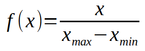
Image 01
This might seem like nonsense. But keep one thing in mind: we can change the value of < x > simply by changing the range. In this case, we will not specify a particular value, but will map it to a particular range of values. At first glance, this expression may not make much sense. So, let's take a closer look at it. Perhaps that will make it a little clearer to you.
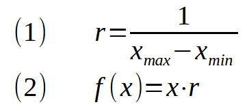
Image 02
Expression (1) shows by how much we will change the scale. If the value of < r > in expression (2) is less than one, the values will be compressed. If it is greater than one, the values will be stretched. It's like zooming in or out within the system.
In the case of a logarithmic scale, the expression will be slightly different, as you've probably already guessed. The fact is that we can use any base to represent data. However, base 10 or base e is generally used, with base e giving the natural logarithm, denoted by ln. I might not even explain this aspect of the logarithmic scale, since from a programming perspective, it's very similar to what we'll be covering here.
Now, to move on to the practical part and make sense of what we've discussed, let's take the code from the previous article and change only the training data. We won't be doing anything else. It's important that you see and understand that this will be the only change. So, in the source code, we have the following snippet:
//+------------------------------------------------------------------+
//Training expression: f(x) = (w0 * 1.8) + (w1 * 2.15) + 2.1
//+------------------------------------------------------------------+
double Train[] {
                  1,    3,  10.35,
                1.5,  3.25, 11.7875,
                1.75, 3.94, 13.721,
                2.85, 3.46, 14.669
               };
//+------------------------------------------------------------------+
#define nColumns    3
#define nLines      Train.Size() / nColumns
//+------------------------------------------------------------------+
Snippet 01
This snippet will be replaced with the following:
//+------------------------------------------------------------------+
//Training expression: f(x) = (w0 * 1.8) + (w1 * 1.254) + (w2 * 2.35) + 4.1258
//+------------------------------------------------------------------+
double Train[] {
                5.89,   12.473, 18.452,  73.731142,
                8.452,  13.154, 24.2541, 92.831651,
                7.512,  14.576, 15.831,  73.128554,
                3.452,  8.459,  30.1254, 91.741676
               };
//+------------------------------------------------------------------+
#define nColumns    4
#define nLines      Train.Size() / nColumns
//+------------------------------------------------------------------+
Snippet 02
01. //+------------------------------------------------------------------+
02. #property copyright "Daniel Jose"
03. #property script_show_inputs
04. #property description   "Script to compare execution speed\n" \
05.                         "Here we are using only the CPU.\n" \
06.                         "However, the results are still very interesting."
07. //+------------------------------------------------------------------+
08. #include <Neural Network\C_Check_Neuron.mqh>
09. //+------------------------------------------------------------------+
10. enum eFactorization {
11.                         Minimum_Square,
12.                         Gradient_Descent,
13.                     };
14. //+------------------------------------------------------------------+
15. input eFactorization        user00 = Minimum_Square;        //Factorization Type
16. input double                user01 = 1e-3;                  //Target error
17. input double                user02 = 1e-3;                  //Learning rate
18. input C_Neuron::eFnActivate user03 = C_Neuron::Identity;    //Activation Function
19. input ulong                 user04 = 5;                     //Number of iterations
20. //+------------------------------------------------------------------+
21. //Training expression: f(x) = (w0 * 1.8) + (w1 * 1.254) + (w2 * 2.35) + 4.1258
22. //+------------------------------------------------------------------+
23. double Train[] {
24.                 5.89,       12.473, 18.452,  73.731142,
25.                 8.452,      13.154, 24.2541, 92.831651,
26.                 7.512,      14.576, 15.831,  73.128554,
27.                 3.452,      8.459,  30.1254, 91.741676
28.                };
29. //+------------------------------------------------------------------+
30. #define nColumns    4
31. #define nLines      Train.Size() / nColumns
32. //+------------------------------------------------------------------+
33. void OnStart()
34. {
35.     C_Check_Neuron *neuron;
36.
37.     Print("************************************");
38.     Print("Simple Neuron in Class...");
39.     Print("************************************");
40.     Print("Parameters:");
41.     Print("Type of factorization: ", EnumToString(user00));
42.     Print("Estimated error: ", user01);
43.     Print("Learning Rate:", user02);
44.     Print("Activation function: ", EnumToString(user03));
45.     Print("Number of interactions: ", user04);
46.     Print("************************************");
47.
48.     neuron = new C_Check_Neuron(nColumns - 1, user03, user00 == Minimum_Square);
49.
50.     (*neuron).View_Training_Data(Train, nColumns);
51.     (*neuron).Performs_Training(Train, user01, user02, user04);
52.     // (*neuron).Check_Training(Train, nColumns);
53.
54.     delete neuron;
55. }
56. //+------------------------------------------------------------------+
Code 01
Note that, in addition to the modified training array, we also have line 19. It allows you to set the number of iterations the code will perform. For practical reasons, line 52, which is responsible for outputting the results, has been commented out, so it will not be executed. However, that isn't so important, because what we really need is for line 51 to execute: that's the one that will show the perceptron's error given this number of iterations. Now let's see what happens when we run this code in the MetaTrader 5 terminal. The result is shown in the image below.
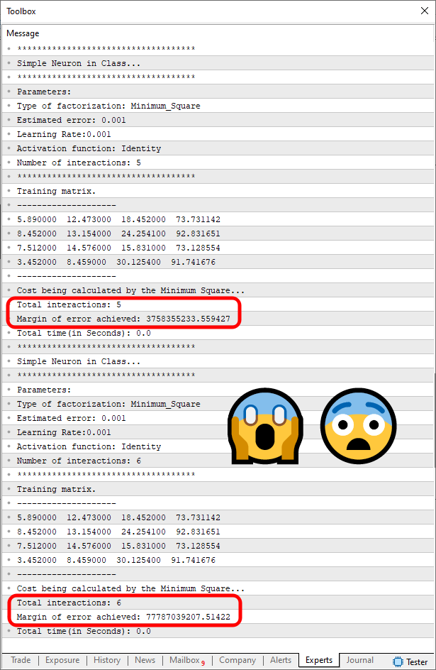
Image 03
To make it easier to understand, I've marked the exact spot where you can see the error displayed by the perceptron. And, to your surprise, take a look: the error didn't decrease—on the contrary, it increased significantly. This means that the perceptron cannot process data from the training array. But why? If you change the values, you'll see that the perceptron works. But when we go beyond certain limits, it seems to go a little crazy, completely lose its bearings, and have no idea which way to go.
This is one of the problems that will require us to change the scale of values. Please pay attention to what I just said. I'm not saying you need to look for suitable values to use. I'm telling you that you need to trick the perceptron into believing it's dealing with one thing, when in fact it's dealing with another.
There are several ways to do this, and each has its own purpose and a very specific goal. But here, since our goal is to make the explanation as clear as possible, we will use a particularly convenient method of explanation. We'll make sure that the application itself—which, in this case, is a script for MetaTrader 5—adjusts the values so that the "dumb" perceptron doesn't realize that things are actually different. To do this, let's move on to the code for the C_Check_Neuron class.
Just a quick note: in the attached file, I'll include the original code so you can reproduce the results exactly as shown in the image above, as well as the code we're about to implement. This will help you understand in practice how and why we need to do things exactly this way.
01. //+------------------------------------------------------------------+
02. #property copyright "Daniel Jose"
03. //+------------------------------------------------------------------+
04. #include <Neural Network\C_Neuron.mqh>
05. //+------------------------------------------------------------------+
06. class C_Check_Neuron : private C_Neuron
07. {
08. //+------------------------------------------------------------------+
09.     private :
10. //+------------------------------------------------------------------+
11.         struct st_0
12.         {
13.             double  Hi,
14.                     Lo,
15.                     Reason;
16.             uint    nColumns,
17.                     nLines;
18.         }m_Limits;
19.         double m_arr[];
20. //+------------------------------------------------------------------+
21.     public  :
22. //+------------------------------------------------------------------+
23.         C_Check_Neuron(const double &arr[], uint nInputs = 1, eFnActivate fn = Identity, bool isFx = false)
24.             :C_Neuron(nInputs, fn, isFx)
25.         {
26.             ZeroMemory(m_Limits);
27.             m_Limits.nColumns = nInputs + 1;
28.             m_Limits.nLines = arr.Size() / m_Limits.nColumns;
29.             m_Limits.Lo = m_Limits.Hi = arr[0];
30.             for (ulong c = 1, m = arr.Size(); c < m; c++)
31.             {
32.                 m_Limits.Hi = MathMax(arr[c], m_Limits.Hi);
33.                 m_Limits.Lo = MathMin(arr[c], m_Limits.Lo);
34.             };
35.             ArrayResize(m_arr, arr.Size());
36.             m_Limits.Reason = 1 / (m_Limits.Hi - m_Limits.Lo);
37.             for (ulong c = 0, m = arr.Size(); c < m; c++)
38.                 m_arr[c] = arr[c] * m_Limits.Reason;
39.         }
40. //+------------------------------------------------------------------+
41.         ~C_Check_Neuron()
42.         {
43.             ArrayFree(m_arr);
44.         }
45. //+------------------------------------------------------------------+
46.         void View_Training_Data(void)
47.         {
48.             string sz0;
49.
50.             Print("Training matrix.");
51.             Print("--------------------");
52.             for (uchar i = 0; i < m_Limits.nLines; i++)
53.             {
54.                 sz0 = "";
55.                 for (uchar j = 0; j < m_Limits.nColumns; j++)
56.                     sz0 += StringFormat("%f  ", m_arr[(i * m_Limits.nColumns) + j]);
57.                 Print(sz0);
58.             }
59.             Print("--------------------");
60.         }
61. //+------------------------------------------------------------------+
62.         void Performs_Training(double epsilon, double LearningRate, ulong limit)
63.         {
64.             ulong it0, it1;
65.
66.             it0 = GetTickCount();
67.             Print("Margin of error achieved: ", Learning(m_arr, epsilon, LearningRate, limit));
68.             it1 = GetTickCount();
69.             Print("Total time(in Seconds): ", (it1 - it0) / 1000.0);
70.         }
71. //+------------------------------------------------------------------+
72.         void Check_Training(const double &arr[])
73.         {
74.             string  sz0;
75.             double  mem[];
76.
77.             Print("********** RESULT *************");
78.             ArrayResize(mem, m_Limits.nColumns);
79.             for (uchar i = 0; i < m_Limits.nLines; i++)
80.             {
81.                 sz0 = "";
82.                 for (uchar j = 0; j < m_Limits.nColumns - 1; j++)
83.                     sz0 += StringFormat("%f  ", mem[j] = arr[(i * m_Limits.nColumns) + j]);
84.                 sz0 += StringFormat("%f", Perceptron(mem));
85.                 Print(sz0);
86.             }
87.             Print("--------------------");
88.             ArrayFree(mem);
89.             View_Variables();
90.         }
91. //+------------------------------------------------------------------+
92. };
93. //+------------------------------------------------------------------+
Code 02
This code isn't finished yet, and there's still a small issue with it. But we'll look at that in more detail later. First, note that a structure has been added on the eleventh line. Its goal is to create a mechanism that we will use to trick the "stupid" perceptron. Please note that an array is declared on the nineteenth line. And now comes the most interesting part. On line 23, where the constructor now takes an array, we'll need to use this new training array.
Now, take a look at what we're about to do. First, on line 26, we clear the memory area where the data structure is located. Next, we initialize some values in this structure; we clear the memory beforehand to avoid working with garbage values. Even if we assign values later, it's always worth making sure the memory is cleared, because we might forget to assign one of them, which would complicate things. And now the most interesting part begins. On line 29, we initialize the maximum and minimum values, and immediately afterward, we enter a loop that will iterate through the entire training array to find the largest and smallest values it contains.
Then, on line 35, we allocate memory for the class's internal array. On line 36, we use the equation we discussed earlier in this article to create an arithmetic scale. So, on line 37, we enter a new loop. But this time, we'll create a transformed training array based on the original training array. That completes the constructor.
//+------------------------------------------------------------------+
void OnStart()
{
    C_Check_Neuron *neuron;

    Print("************************************");
    Print("Simple Neuron in Class...");
    Print("************************************");
    Print("Parameters:");
    Print("Type of factorization: ", EnumToString(user00));
    Print("Estimated error: ", user01);
    Print("Learning Rate:", user02);
    Print("Activation function: ", EnumToString(user03));
    Print("Number of interactions: ", user04);
    Print("************************************");

    neuron = new C_Check_Neuron(Train, nColumns - 1, user03, user00 == Minimum_Square);

    (*neuron).View_Training_Data();
    (*neuron).Performs_Training(user01, user02, user04);
    // (*neuron).Check_Training(Train);

    delete neuron;
}
//+------------------------------------------------------------------+
Snippet 03
Here, I'll highlight only the part of the code that has changed. There is nothing here that requires an explanation, given how simple it is. But now let's see what happens when we compile and run this code in the MetaTrader 5 terminal. The result is shown in the image below.
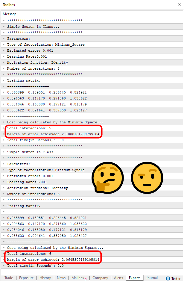
Image 04
"What on earth is this? It must be a miracle. How come the perceptron now understands the situation and has started to converge? What on earth just happened?" My friend, there are some things you can only understand and believe once you've seen them with your own eyes. If you simply told people about this, no one would believe you; they'd say you had no idea what you were talking about, or at least didn't understand what you were doing. But you can clearly see that the perceptron has changed its behavior. And all this is simply because we changed the scale of values. Well, isn't that crazy? And yet there are still people who think they've seen it all in this life. I say: “You don't know anything, you naive soul.”
45. //+------------------------------------------------------------------+
46.         void View_Training_Data(void)
47.         {
48.             string sz0;
49.
50.             Print("Training matrix.");
51.             Print("--------------------");
52.             for (uchar i = 0; i < m_Limits.nLines; i++)
53.             {
54.                 sz0 = "";
55.                 for (uchar j = 0; j < m_Limits.nColumns; j++)
56.                     sz0 += StringFormat("%f  ", m_arr[(i * m_Limits.nColumns) + j] / m_Limits.Reason);
57.                 Print(sz0);
58.             }
59.             Print("--------------------");
60.         }
61. //+------------------------------------------------------------------+
Snippet 04
All right, now let's compile and run the code again. We will get the following result, shown in the image below:
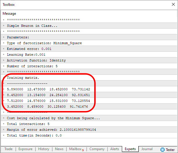
Image 05
Now that's more like it. Not only are we tricking this dumb and silly perceptron, but we're also giving the user the impression that everything is perfectly fine. But we still have one more problem. To identify this new issue, you need to re-enable the code that displays the results. In addition to allowing the perceptron to converge to a more appropriate error value—since we now know that it does indeed converge—we can remove the option for user configuration and leave the code as shown below.
//+------------------------------------------------------------------+
void OnStart()
{
    C_Check_Neuron *neuron;

    Print("************************************");
    Print("Simple Neuron in Class...");
    Print("************************************");
    Print("Parameters:");
    Print("Type of factorization: ", EnumToString(user00));
    Print("Estimated error: ", user01);
    Print("Learning Rate:", user02);
    Print("Activation function: ", EnumToString(user03));
    Print("************************************");

    neuron = new C_Check_Neuron(Train, nColumns - 1, user03, user00 == Minimum_Square);

    (*neuron).View_Training_Data();
    (*neuron).Performs_Training(user01, user02, ULONG_MAX);
    (*neuron).Check_Training(Train);

    delete neuron;
}
//+------------------------------------------------------------------+
Code 03
Once again, we compile and run the new version of the code, and the result in the MetaTrader 5 terminal will be as follows:
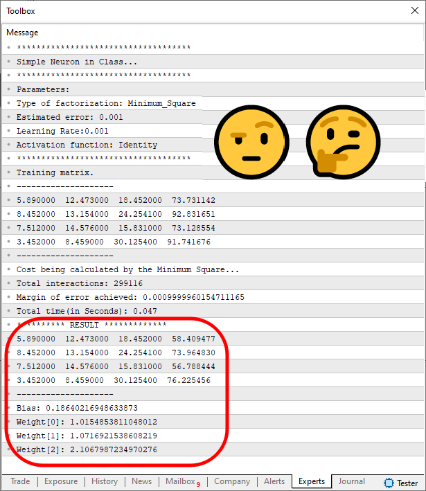
Image 06
"But wait a minute. That's wrong. What happened to make the result turn out so badly?" Well, dear reader, a programmer's life isn't always perfect and peaceful. Sometimes we need to understand what we're doing; otherwise, we end up with an answer that we don't understand ourselves. And, because we don't understand it, we end up rejecting the solution, even when it isn't as wrong as it might seem at first glance. For this reason, we will try to figure out what happened, since the result differed so greatly from what we expected.
To do this, we need to use a math software package that allows us to plot a graph. That will make it easier to understand what's going on here. I will use the code below in SciLab, which is free software, although MATLAB could also be used. Both programs produce the same type of result.
clc;
clear;
clf;

x = [-2:0.01:2];
y =  (1.8 * x) + (1.254 * x) + (2.35 * x) + 4.1258;
plot(x, y, 'p-');

y = (1.0154853811048012 * x) + (1.0716921538608219 * x) + (2.1067987234970276 * x) + 0.18640216948633873;
plot(x, y, 'r-');

xgrid(0, 1);
SciLab Script
The result is shown below.
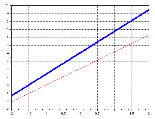
Image 07
//+------------------------------------------------------------------+
        inline double Learning(const double &train[], double reason, double epsilon, double LearningRate, ulong limit = ULONG_MAX)
        {
           double err = (m_Infos.IsFx ? Learning_FX(train, epsilon, LearningRate, limit) : Learning_DX(train, epsilon, LearningRate, limit));

           m_Infos.Bias /= reason;

           return err;
        }
 //+------------------------------------------------------------------+
Snippet 05
//+------------------------------------------------------------------+
        void Performs_Training(double epsilon, double LearningRate, ulong limit)
        {
            ulong it0, it1;

            it0 = GetTickCount();
            Print("Margin of error achieved: ", Learning(m_arr, m_Limits.Reason, epsilon, LearningRate, limit));
            it1 = GetTickCount();
            Print("Total time(in Seconds): ", (it1 - it0) / 1000.0);
        }
//+------------------------------------------------------------------+
Snippet 06
That's how we solve part of the problem. Now let's run the script again and get the following result.
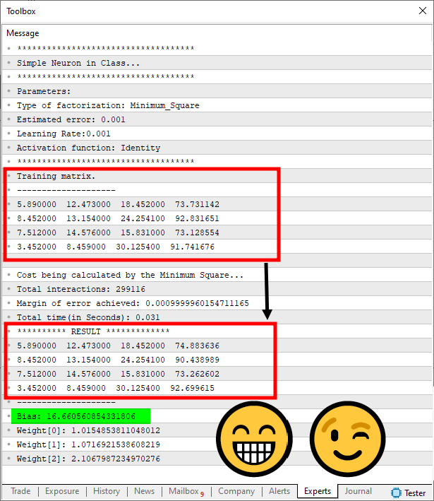
Image 08
clc;
clear;
clf;

x = [-2:0.01:2];
y =  (1.8 * x) + (1.254 * x) + (2.35 * x) + 4.1258;
plot(x, y, 'p-');

y = (1.0154853811048012 * x) + (1.0716921538608219 * x) + (2.1067987234970276 * x) + 0.18640216948633873;
plot(x, y, 'r-');


y = (1.0154853811048012 * x) + (1.0716921538608219 * x) + (2.1067987234970276 * x) + 16.660560854331806;
plot(x, y, 'g-');


xgrid(0, 1);
SciLab Script
We will obtain the following graph.
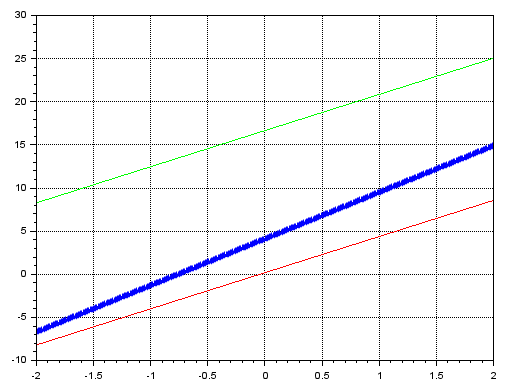
Image 09
Note that the green line shows the values obtained after adjusting the bias. Although these values may be appropriate for some situations, they may not be suitable for many others. So, to try to improve the situation a little more, we'll change the target (expected) error value and the learning rate. Since the default values are on the order of 1e-3, let's try using 1e-5 for both the target (expected) error and the learning rate. We'll get the result shown in the image below:
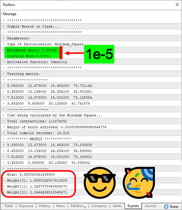
Image 10
clc;
clear;
clf;

x = [-2:0.25:2];
y =  (1.8 * x) + (1.254 * x) + (2.35 * x) + 4.1258;
plot(x, y, 'p-');

y = (1.0154853811048012 * x) + (1.0716921538608219 * x) + (2.1067987234970276 * x) + 0.18640216948633873;
plot(x, y, 'r-');


y = (1.0154853811048012 * x) + (1.0716921538608219 * x) + (2.1067987234970276 * x) + 16.660560854331806;
plot(x, y, 'g-');

y = (1.6580026007613309 * x) + (1.3267078963939070 * x) + (2.3446624518945471 * x) + 4.258060261635903;
plot(x, y, 'mo');

xgrid(0, 1);
SciLab Script
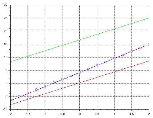
Image 11
Here's something interesting to note. The blue line shows the actual training data. The green line shows the error value when we train with both the target (expected) error and the learning rate set to 1e-3. The small purple circles show the result when we use the same code but with a value of 1e-5. This result is truly surprising.
Concluding Thoughts
In this article, I have shown that we still have a lot to learn before we can assume that we already know everything. I have mentioned more than once that, despite all its achievements, HUMANITY STILL DOES NOT KNOW HOW TO CREATE THE ULTIMATE PERCEPTRON NETWORK. We conduct research and try to learn from our own successes and mistakes.
I'm not here to disparage or insult anyone, and I don't even need to prove anything to anyone. I'm just here to share my experience as a programmer. And, as this article makes clear, it is not enough to simply collect a dataset to create something that can truly mimic the human mind.
There are some details that many people aren't aware of. But after reading this article, you already understand that we often have to tweak the code to turn data that seems disjointed at first glance into something truly usable.
| MQ5 File | Description |
|---|---|
| Scripts\Example A | Basic Demonstration |
Translated from Portuguese by MetaQuotes Ltd.
Original article: https://www.mql5.com/pt/articles/13942
Warning: All rights to these materials are reserved by MetaQuotes Ltd. Copying or reprinting of these materials in whole or in part is prohibited.
This article was written by a user of the site and reflects their personal views. MetaQuotes Ltd is not responsible for the accuracy of the information presented, nor for any consequences resulting from the use of the solutions, strategies or recommendations described.