Neural Networks in Practice: The Perceptron
 48
 0

Introduction
In our previous article, “Neural Networks in Practice: The Gradient”, we briefly discussed how the gradient arises from the use of the derivative of the loss function.
Although breaking this material down into parts is no easy task—since the topic requires familiarity with a vast number of elements and concepts, many of which are entirely abstract, while others are quite complex due to the use of the same terms in different contexts—I have tried to present the material as clearly as possible.
Among these concepts are the terms “backpropagation” and “forward propagation,” which are often confused or used interchangeably, usually without proper explanation. To fully understand everything that happens in the code of a perceptron network, we need to understand how these concepts came about.
For now, we won't go into certain details. However, we need to understand how the term “neural network” came about. To do this, we need to understand the basic building block known as a perceptron—which is the main topic of this article.
Perceptron
When the topic of perceptrons comes up, many people immediately start thinking about artificial intelligence. The term itself was coined by McCulloch and Pitts, and in 1958, Frank Rosenblatt put this idea into practice while working at the Cornell Aeronautical Laboratory. Rosenblatt drew inspiration from the biological neuron and what it is capable of. Essentially, a perceptron consists of one or more inputs, a processing unit, and an output that represents the result of that processing.
However, the first practical implementation was carried out on the IBM 704, where Rosenblatt attempted to use software to create a system capable of recognizing faces. It is interesting to note that the following phrase was used in the description of that perceptron: “A perceptron is the embryo of an electronic computer that, the Navy hopes, will be able to walk, talk, see, write, reproduce, and be aware of its own existence.” These people are just a joke. I can only imagine how much money they must have received for research after that demonstration.
Due to technical difficulties, the system did not function as expected and was only able to process linear patterns. For this reason, the system was unable to recognize other patterns as intended. As a result, interest in artificial intelligence research faded away for a while.
A perceptron uses several input values. Using weights and a bias, it can perform weighted addition and multiplication. The name proved quite interesting, since the function being developed could perform exactly this kind of task. In other words, if we feed several input values into the function and it has previously acquired knowledge, it will be able to perform tasks of the same type.
This same function could perform all the necessary additions and multiplications, thereby forming a kind of identity template. Thus, by passing the output signal through a function that came to be called an activation function—specifically to distinguish the output function from the perceptron's internal transformation—we ultimately obtained an output signal that could be fed to other perceptrons or displayed to us humans.
In a future article, I will explain how the original idea behind the perceptron function came about: precisely this chain of weighted additions and multiplications. But we'll come back to that later, since it requires an understanding of certain concepts that many people might not be interested in exploring right now.
So, let's get back to the topic and take a look at the perceptron from a more modern perspective. For simplicity's sake, let's focus on a single perceptron for now. Although in previous articles we have already begun connecting perceptrons in a chain to model logic gates, the goal here is to introduce you to a slightly more complex form of modeling.
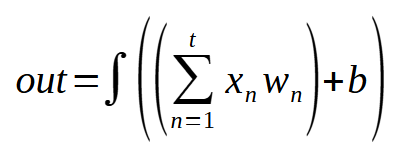
Essentially, a perceptron uses the mathematical expression we discussed in the previous article. You can see it again below.
 //+------------------------------------------------------------------+
        inline double Perceptron(const double &inputs[])
        {
            double value = m_Infos.Bias;

            for (uint c = 0; c < m_Infos.nInputs; c++)
                value += (inputs[c] * m_Infos.Weight[c]);

            return fnActivation(true, value);
        }
//+------------------------------------------------------------------+
This code snippet contains virtually everything that has been implemented in the C_Neuron class so far, with one exception: the fnActivation function, which has not yet been fully implemented. Aside from this detail, it's clear that we're simply performing addition and multiplication. That's it.
Contrary to what the previous article might have suggested, a perceptron is nothing more than a sequence of simple additions and multiplications. However, once we set the constants in the mathematical expression, we can obtain a result that may turn out to be interesting. These constants, which correspond to the values of the weights and the bias, are adjusted during the so-called training process. Thus, the main goal of any network is to adjust these constants, and that is exactly the purpose of the function we call a perceptron.
So, now that we understand this, we can take a look at the function that is currently missing from the code—namely, fnActivation, shown below.
//+------------------------------------------------------------------+
        inline double fnActivation(const bool isFx, const double value)
        {
            switch (m_Infos.Activate)
            {
                case Sigmoid:
                        return (isFx ? 1 / (1 + MathExp(-value)) : MathExp(-value) / MathPow(1 + MathExp(-value), 2));
                case Tangh:
                        return (isFx ? (2 / (1 + MathExp(-2 * value))) - 1 : (4 / MathPow(MathExp(-value) + MathExp(value), 2)));
                case ReLU:
                        return (isFx ? MathMax(0, value) : (value <= 0 ? 0 : 1));
                case eLU:
                        return (isFx ? (value <= 0 ? (m_Infos.Alpha * (MathExp(value) - 1)) : value) : (value <= 0 ? (m_Infos.Alpha * MathExp(value)) : 1));
                case SoftSign:
                        return (isFx ? value / (1 + MathAbs(value)) : value / MathPow(1 + MathAbs(value), 2));
                case SoftPlus:
                        return (isFx ? MathLog(1 + MathExp(value)) : 1 / (1 + MathExp(-value)));
                case Identity:
                default:
                        return (isFx ? value : 1);
            }
        }
//+------------------------------------------------------------------+
Now we have a general idea of how a complete perceptron works and what it can do. This is because the activation functions presented here are the same ones that were shown and discussed in the article where we explained them using graphs. But note one thing: although we have all the functions shown above, you may notice that the perceptron does not use derivatives. This is because the isFx parameter never takes the value false. Why do we calculate the derivative here? The answer lies in the gradient. But before we get into that, I want you to understand one thing.
The activation function in the least squares method
To understand how it really works, we need to look at it in its simplest form. Since our C_Neuron class already has some functionality, we will focus on the complete code for the class. That will make it easier to explain and, most importantly, to understand what's going on. The code itself is shown below.
//+------------------------------------------------------------------+
#property copyright "Daniel Jose"
//+------------------------------------------------------------------+
#define macroRandom (rand() / (double)SHORT_MAX)
//+------------------------------------------------------------------+
class C_Neuron
{
    protected:
//+------------------------------------------------------------------+
        enum eFnActivate {
                            Identity,
                            Sigmoid,
                            Tangh,
                            SoftSign,
                            ReLU,
                            eLU,
                            SoftPlus,
                        };
//+------------------------------------------------------------------+
    private:
//+------------------------------------------------------------------+
        struct  stInfos
        {
            bool    IsFx;
            uint    nInputs;
            double  Bias,
                    Weight[],
                    Alpha;
            eFnActivate Activate;
        }m_Infos;
//+------------------------------------------------------------------+
        struct stErr
        {
            double  weight[],
                    eMaxWeight,
                    bias;
        }m_Error;
//+------------------------------------------------------------------+
        inline double fnActivation(const bool isFx, const double value)
        {
            switch (m_Infos.Activate)
            {
                case Sigmoid:
                        return (isFx ? 1 / (1 + MathExp(-value)) : MathExp(-value) / MathPow(1 + MathExp(-value), 2));
                case Tangh:
                        return (isFx ? (2 / (1 + MathExp(-2 * value))) - 1 : (4 / MathPow(MathExp(-value) + MathExp(value), 2)));
                case ReLU:
                        return (isFx ? MathMax(0, value) : (value <= 0 ? 0 : 1));
                case eLU:
                        return (isFx ? (value <= 0 ? (m_Infos.Alpha * (MathExp(value) - 1)) : value) : (value <= 0 ? (m_Infos.Alpha * MathExp(value)) : 1));
                case SoftSign:
                        return (isFx ? value / (1 + MathAbs(value)) : value / MathPow(1 + MathAbs(value), 2));
                case SoftPlus:
                        return (isFx ? MathLog(1 + MathExp(value)) : 1 / (1 + MathExp(-value)));
                case Identity:
                default:
                        return (isFx ? value : 1);
            }
        }
//+------------------------------------------------------------------+
        inline double Cost_FX(const double &train[])
        {
            double x, err;

            err = 0;
            for (uint c0 = 0; c0 < train.Size(); c0++)
            {
                x = 0;
                for(uint c1 = 0; c1 < m_Infos.nInputs; c1++, c0++)
                   x += (train[c0] * m_Infos.Weight[c1]);
                err += MathPow((x + m_Infos.Bias) - train[c0], 2);
            }

            return err;
        }
//+------------------------------------------------------------------+
        inline double Learning_FX(const double &train[], const double epsilon,  const double LearningRate, const ulong limit)
        {
            double  err,
                    memT,
                    err_w[];
            ulong   count;

            Print("Cost being calculated by the Minimum Square...");
            ArrayResize(err_w, m_Infos.nInputs);
            for (count = 0; (count < limit) && ((err = Cost_FX(train)) > epsilon); count++)
            {
                for (uint c = 0, m = m_Infos.Weight.Size(); c < m; c++)
                {
                    memT = m_Infos.Weight[c];
                    m_Infos.Weight[c] += LearningRate;
                    err_w[c] = Cost_FX(train) - err;
                    m_Infos.Weight[c] = memT;
                }
                memT = m_Infos.Bias;
                m_Infos.Bias += LearningRate;
                m_Infos.Bias = memT - (Cost_FX(train) - err);
                for (uint c = 0, m = m_Infos.Weight.Size(); c < m; c++)
                    m_Infos.Weight[c] -= err_w[c];
            }
            PrintFormat("Total interactions: %I64u", count);
            ArrayFree(err_w);

            return err;
        }
//+------------------------------------------------------------------+
        inline double Cost_DX(const double &train[])
        {
            double  x1, t;

            ZeroMemory(m_Error);
            for (uint c0 = 0, cw = 0; c0 < train.Size(); c0++, cw = c0)
            {
                x1 = 0;
                for(uint c1 = 0; c1 < m_Infos.nInputs; c1++, c0++)
                   x1 += (train[c0] * m_Infos.Weight[c1]);
                t = 2 * ((x1 + m_Infos.Bias) - train[c0]);
                for(uint c1 = 0; c1 < m_Infos.nInputs; c1++, cw++)
                {
                    m_Error.weight[c1] += (t * train[cw]);
                    m_Error.eMaxWeight = (MathAbs(m_Error.weight[c1]) >  MathAbs(m_Error.eMaxWeight) ? m_Error.weight[c1] : m_Error.eMaxWeight);
                }
                m_Error.bias += t;
            }
            return (MathAbs(m_Error.bias) > MathAbs(m_Error.eMaxWeight) ? m_Error.bias : m_Error.eMaxWeight);
        }
//+------------------------------------------------------------------+
        inline double Learning_DX(const double &train[], const double epsilon, const double LearningRate, const ulong limit)
        {
            ulong   count;
            double  eRet;

            Print("Cost being calculated by the Gradient...");
            for (count = 0; (count < limit) && (MathAbs(eRet = Cost_DX(train)) > epsilon); count++)
            {
                m_Infos.Bias -= (m_Error.bias * LearningRate);
                for (uint c = 0, m = m_Infos.Weight.Size(); c < m; c++)
                    m_Infos.Weight[c] -= (m_Error.weight[c] * LearningRate);
            }
            PrintFormat("Total interactions: %I64u", count);

            return eRet;
        }
//+------------------------------------------------------------------+
    public :
//+------------------------------------------------------------------+
        C_Neuron(uint nInputs = 1, eFnActivate fn = Identity, bool isFx = false, double alpha = 0.75, double H = 1.0, double L = 0.0)
        {
            MathSrand(512);
            ZeroMemory(m_Infos);
            m_Infos.Activate = fn;
            m_Infos.IsFx = isFx;
            m_Infos.Alpha = alpha;
            m_Infos.Bias = (double)macroRandom;
            ArrayResize(m_Infos.Weight, m_Infos.nInputs = nInputs);
            ArrayResize(m_Error.weight, m_Infos.nInputs);
            for(uint c = 0; c < m_Infos.nInputs; c++)
                m_Infos.Weight[c] = ((double)macroRandom * (H - L)) + L;
        }
//+------------------------------------------------------------------+
        ~C_Neuron()
        {
            ArrayFree(m_Infos.Weight);
            ArrayFree(m_Error.weight);
        }
//+------------------------------------------------------------------+
        void View_Variables(void)
        {
            Print("Bias: ", m_Infos.Bias);
            for (uint c = 0, m = m_Infos.Weight.Size(); c < m; c++)
                PrintFormat("Weight[%d]: %.16f", c, m_Infos.Weight[c]);
        }
//+------------------------------------------------------------------+
        inline double Learning(const double &train[], const double epsilon = 1e-3, const double LearningRate = 1e-2, const ulong limit = ULONG_MAX)
        {
           return (m_Infos.IsFx ? Learning_FX(train, epsilon, LearningRate, limit) : Learning_DX(train, epsilon, LearningRate, limit));
        }
 //+------------------------------------------------------------------+
        inline double Perceptron(const double &inputs[])
        {
            double value = m_Infos.Bias;

            for (uint c = 0; c < m_Infos.nInputs; c++)
                value += (inputs[c] * m_Infos.Weight[c]);

            return fnActivation(true, value);
        }
//+------------------------------------------------------------------+
};
//+------------------------------------------------------------------+
#undef macroRandom
//+------------------------------------------------------------------+
I know that showing all the code might seem silly, but I want to demonstrate something to you. You'll find the finished code in the attached file. However, seeing what everything looked like before is just as important—and in some cases even more important—than seeing the final code. Please take note of this so you can understand how it needs to be changed. This will help you understand why the code will behave that way later on.
Here, only the perceptron uses an activation function. Neither the loss function using the least squares method nor the function using the gradient is called here.
Now, pay attention: before we make any changes to the C_Neuron class, let's create another class. It will help reduce the amount of code during testing by consolidating everything into a single header file. The class we are going to create is shown in full below.
//+------------------------------------------------------------------+
#property copyright "Daniel Jose"
//+------------------------------------------------------------------+
#include <Neural Network\C_Neuron.mqh>
//+------------------------------------------------------------------+
class C_Check_Neuron : private C_Neuron
{
//+------------------------------------------------------------------+
    private :
//+------------------------------------------------------------------+
    public  :
//+------------------------------------------------------------------+
        C_Check_Neuron(uint nInputs = 1, eFnActivate fn = Identity, bool isFx = false)
            :C_Neuron(nInputs, fn, isFx)
        {}
//+------------------------------------------------------------------+
        void View_Training_Data(const double &arr[], uint nColumns)
        {
            string sz0;
            uint nLines = arr.Size() / nColumns;

            Print("Training matrix.");
            Print("--------------------");
            for (uchar i = 0; i < nLines; i++)
            {
                sz0 = "";
                for (uchar j = 0; j < nColumns; j++)
                    sz0 += StringFormat("%f  ", arr[(i * nColumns) + j]);
                Print(sz0);
            }
            Print("--------------------");
        }
//+------------------------------------------------------------------+
        void Performs_Training(const double &arr[], double epsilon, double LearningRate, ulong limit)
        {
            ulong it0, it1;

            it0 = GetTickCount();
            Print("Margin of error achieved: ", Learning(arr, epsilon, LearningRate, limit));
            it1 = GetTickCount();
            Print("Total time(in Seconds): ", (it1 - it0) / 1000.0);
        }
//+------------------------------------------------------------------+
        void Check_Training(const double &arr[], uint nColumns)
        {
            string  sz0;
            double  mem[];
            uint    nLines = arr.Size() / nColumns;

            Print("********** RESULT *************");
            ArrayResize(mem, nColumns);
            for (uchar i = 0; i < nLines; i++)
            {
                sz0 = "";
                for (uchar j = 0; j < nColumns - 1; j++)
                    sz0 += StringFormat("%f  ", mem[j] = arr[(i * nColumns) + j]);
                sz0 += StringFormat("%f", Perceptron(mem));
                Print(sz0);
            }
            Print("--------------------");
            ArrayFree(mem);
            View_Variables();
        }
//+------------------------------------------------------------------+
};
//+------------------------------------------------------------------+
The C_Check_Neuron class will allow us to output data, run training, and verify the results. Since this class contains only the essentials we'll need later, it will be easier to follow the explanation without getting lost. Now let's take a look at the first of the code snippets we'll use to test the perceptron. The code is shown below.
//+------------------------------------------------------------------+
#property copyright "Daniel Jose"
#property script_show_inputs
#property description   "Script to compare execution speed\n" \
                        "Here we are using only the CPU.\n" \
                        "However, the results are still very interesting."
//+------------------------------------------------------------------+
#include <Neural Network\C_Check_Neuron.mqh>
//+------------------------------------------------------------------+
enum eFactorization {
                        Minimum_Square,
                        Gradient_Descent,
                    };
//+------------------------------------------------------------------+
input eFactorization        user00 = Minimum_Square;        //Calculation type
input double                user01 = 1e-3;                  //Target error
input double                user02 = 1e-3;                  //Learning rate
input C_Neuron::eFnActivate user03 = C_Neuron::Identity;    //Activation function
//+------------------------------------------------------------------+
double Train[] {
                0, 0,
                1, 2,
                2, 4,
                3, 6,
                4, 8
               };
//+------------------------------------------------------------------+
#define nColumns    2
#define nLines      Train.Size() / nColumns
//+------------------------------------------------------------------+
void OnStart()
{
    C_Check_Neuron *neuron;

    Print("************************************");
    Print("Simple Neuron in Class...");
    Print("************************************");
    Print("Parameters:");
    Print("Type of factorization: ", EnumToString(user00));
    Print("Estimated error: ", user01);
    Print("Learning Rate:", user02);
    Print("Activation function: ", EnumToString(user03));
    Print("************************************");


    neuron = new C_Check_Neuron(nColumns - 1, user03, user00 == Minimum_Square);

    (*neuron).View_Training_Data(Train, nColumns);
    (*neuron).Performs_Training(Train, user01, user02, ULONG_MAX);
    (*neuron).Check_Training(Train, nColumns);

    delete neuron;
}
//+------------------------------------------------------------------+
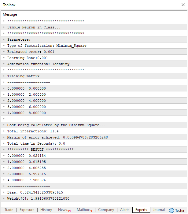
Since most of the complexity has been moved inside the C_Check_Neuron class, the code shown above allows you to run all the tests while outputting the various data needed to understand what the perceptron is doing. In fact, we can even analyze whether convergence to the minimum of the loss function has actually occurred. If you run the code above exactly as written, you'll see something similar to what's shown in the following image.
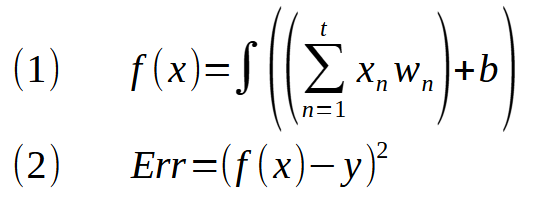
And here we have an activation function applied to the least squares method. Remember that the integral sign actually denotes an activation function included in the expression as a multiplier. Now I want you to compare expression (1) with the perceptron expression. Please note that they are identical. Then you're probably wondering, "How is that possible?" Is there a specific reason why this happens? Yes, my friend. The system, based on perceptron networks, was developed primarily to solve linear regression problems and remains focused on that specific task. If you're not sure what I'm talking about, check out my first few articles on this topic.
There, I explained how this idea came about. But the focus here is on equation (2), not equation (1). Expression (1) represents forward propagation. In turn, expression (2) corresponds precisely to backpropagation, which will be applied to the perceptron. Please note that there isn't much of a difference here compared to what was shown earlier. However, if you look at the code—especially the way I write it—you might get the impression that everything works differently than I show in the mathematical expressions. For this reason, I'm including these expressions so that you can properly understand where each piece of code comes from. Now, to implement this in the code, we add the following snippet to the C_Neuron class.
//+------------------------------------------------------------------+
        inline double Cost_FX(const double &train[])
        {
            double x, err;

            err = 0;
            for (uint c0 = 0; c0 < train.Size(); c0++)
            {
                x = 0;
                for(uint c1 = 0; c1 < m_Infos.nInputs; c1++, c0++)
                   x += (train[c0] * m_Infos.Weight[c1]);
                err += MathPow(fnActivation(true, x + m_Infos.Bias) - train[c0], 2);
            }

            return err;
        }
//+------------------------------------------------------------------+
The difference is very subtle, so you need to pay close attention to catch the moment when the activation function is called. In fact, if you run the test code again, you'll see the image shown below.
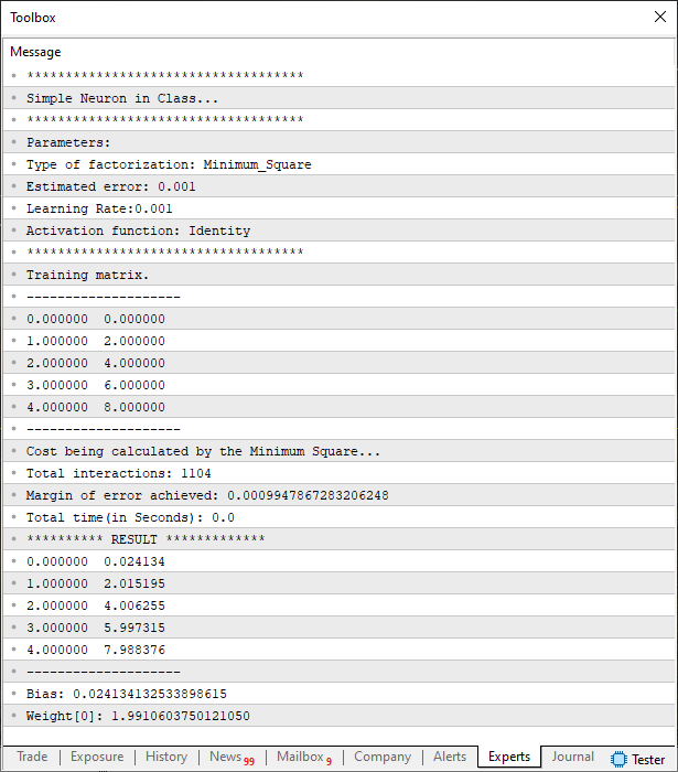
It looks like a repetition of what was done before, but that's not actually the case: these are different points in the execution of the same code. Once with the activation function, and once without it. But pay even closer attention to the fact that we are using the identity activation function. This is because, in this case, we are indeed using linear regression. Using any other activation function would make no sense.
Okay, but can this same perceptron process a different number of inputs? It's easy to see for yourself. To do this, we'll use the code below.
//+------------------------------------------------------------------+
#property copyright "Daniel Jose"
#property script_show_inputs
#property description   "Script to compare execution speed\n" \
                        "Here we are using only the CPU.\n" \
                        "However, the results are still very interesting."
//+------------------------------------------------------------------+
#include <Neural Network\C_Check_Neuron.mqh>
//+------------------------------------------------------------------+
enum eFactorization {
                        Minimum_Square,
                        Gradient_Descent,
                    };
//+------------------------------------------------------------------+
input eFactorization        user00 = Minimum_Square;        //Calculation type
input double                user01 = 1e-3;                  //Target error
input double                user02 = 1e-3;                  //Learning rate
input C_Neuron::eFnActivate user03 = C_Neuron::Identity;    //Activation function
//+------------------------------------------------------------------+
//Training expression: f(x) = (w0 * 1.8) + (w1 * 2.15) + 2.1
//+------------------------------------------------------------------+
double Train[] {
                  1,    3,  10.35,
                1.5,  3.25, 11.7875,
                1.75, 3.94, 13.721,
                2.85, 3.46, 14.669
               };
//+------------------------------------------------------------------+
#define nColumns    3
#define nLines      Train.Size() / nColumns
//+------------------------------------------------------------------+
void OnStart()
{
    C_Check_Neuron *neuron;

    Print("************************************");
    Print("Simple Neuron in Class...");
    Print("************************************");
    Print("Parameters:");
    Print("Type of factorization: ", EnumToString(user00));
    Print("Estimated error: ", user01);
    Print("Learning Rate:", user02);
    Print("Activation function: ", EnumToString(user03));
    Print("************************************");


    neuron = new C_Check_Neuron(nColumns - 1, user03, user00 == Minimum_Square);

    (*neuron).View_Training_Data(Train, nColumns);
    (*neuron).Performs_Training(Train, user01, user02, ULONG_MAX);
    (*neuron).Check_Training(Train, nColumns);

    delete neuron;
}
//+------------------------------------------------------------------+
When you run this code, the following result will be displayed in the terminal.
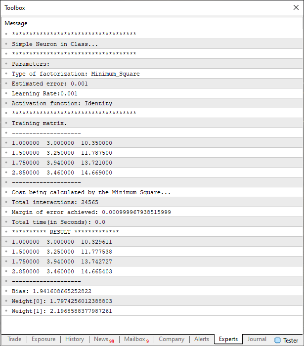
I'm not sure if you're following my line of reasoning. Only a few changes were needed to turn the previous test script into this version. Both scripts are intended to test the perceptron. Specifically, changes were made to the definition specifying the number of columns in the training array, as well as to the data used during training. Therefore, if you want to use completely different data, you won't have any trouble experimenting with this perceptron. However, as already mentioned, we need to take certain precautions. Perhaps the most important thing is the value specified in the learning rate field.
You shouldn't use values that are too high, because that ultimately drives the perceptron a little crazy. You should also avoid using values that are too small, because in that case the perceptron will take a long time to converge and reduce the error below the target value. In other words, the key to success is moderation.
When I say that a perceptron goes a little crazy, I'm referring to a mathematical phenomenon. The issue isn't that there's some kind of bug in the program that causes it to enter an excessively long loop, but rather a mathematical problem related to the convergence of values. To understand this, take a look at the following image.
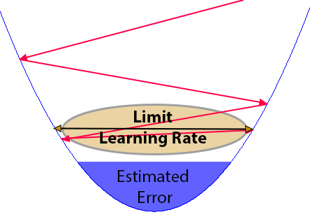
This image, which may seem confusing at first glance, actually illustrates the problem of using an inappropriate learning rate. I usually prefer to set this value so that it is equal to or slightly less than the target error, precisely to avoid the situation shown in the previous image.
As the perceptron converges toward the target error, as shown by the red lines, at some point it may enter a valley where the distance between the slopes is very close to the learning rate. Although the target error value is defined correctly, the distance between the valley slopes causes the perceptron to stop converging, with the result that it does not reach the previously specified error and the process never terminates. This happens because the learning rate can cause the perceptron to swing back and forth, preventing it from even continuing its descent. This is probably the worst-case scenario we could face, since it might seem to you that the app has frozen. Hence the need for some kind of mechanism to get out of such an unpleasant situation.
One of the mechanisms used involves setting the maximum number of training iterations. Personally, I prefer to leave it at ULONG_MAX. However, this could result in the training taking too long. Therefore, when setting the learning rate, one should take into account the target error and, possibly, even the maximum number of training iterations. These settings can be adjusted without changing any of the code provided here; you only need to adjust the settings in the final application's code.
If you found all of this interesting and were able to understand how the activation function is used when we choose the least squares method, then it's time to look at something even more interesting. Now let's see what happens when we select the gradient. But to keep these two topics separate, let's discuss this in a new section.
The Activation Function in Gradient Computation
Now things are going to get a lot more interesting. What we covered in the previous topic is just child's play. But what we're about to see here can be summed up this way: this is where it all begins. That's when the children start crying, because they don't know how to get out of a difficult situation, and they wait for an adult to come and rescue them.
All joking aside, applying the activation function to the gradient isn't as simple as applying it to the loss function in the least squares method. This is precisely because the gradient is the derivative of the least squares loss function. However, there is one detail, and it is precisely because of this detail that many people get confused when trying to understand the gradient. Especially when they start from a misconception without first understanding how the least squares method works.
Unlike the least squares method, whose expressions are practically identical to what we saw in the perceptron, the gradient involves two expressions. One is for the output, and the other is for backpropagation. That's why many people end up getting confused. But there's no reason to worry or panic. Please try to understand what I'm about to explain. You'll see that in practice, it's much easier than it seems. In my previous article, I presented the following expression:

In other words, the error is essentially a set of derivatives when our goal is to use the gradient. Therefore, to begin correcting the error, we simply need to multiply the gradient by the derivative of the activation function. It's that simple. In the following code snippet, you can see how this is implemented.
//+------------------------------------------------------------------+
        inline double Cost_DX(const double &train[])
        {
            double  x1, t;

            ZeroMemory(m_Error);
            for (uint c0 = 0, cw = 0; c0 < train.Size(); c0++, cw = c0)
            {
                x1 = 0;
                for(uint c1 = 0; c1 < m_Infos.nInputs; c1++, c0++)
                   x1 += (train[c0] * m_Infos.Weight[c1]);
                t = 2 * ((x1 + m_Infos.Bias) - train[c0]) * fnActivation(false, x1 + m_Infos.Bias);
                for(uint c1 = 0; c1 < m_Infos.nInputs; c1++, cw++)
                {
                    m_Error.weight[c1] += (t * train[cw]);
                    m_Error.eMaxWeight = (MathAbs(m_Error.weight[c1]) >  MathAbs(m_Error.eMaxWeight) ? m_Error.weight[c1] : m_Error.eMaxWeight);
                }
                m_Error.bias += t;
            }
            return (MathAbs(m_Error.bias) > MathAbs(m_Error.eMaxWeight) ? m_Error.bias : m_Error.eMaxWeight);
        }
//+------------------------------------------------------------------+
"But is that all?" Yes, dear reader, that's all we need to do. Now we have a perceptron that uses the gradient and can also use the least squares method. In general terms, we can say that the perceptron is complete. In other words, we have inputs, a loss function, an activation function, backpropagation, and an output. All of this has already been implemented in our perceptron using the C_Neuron class. All the unnecessary complexity that many people introduce into this topic only makes it seem more complicated than it actually is.
Summary
You may still be somewhat skeptical about whether we really need to use the derivative of the activation function when we use the gradient. To understand why it is necessary, we'll have to look at the mathematical aspects. Therefore, the rest of this article will be devoted to explaining how we arrived at this conclusion and why we need to use derivatives. If you'd like, you can skip the rest of the article. But I assure you that this will be a good review of everything we've covered so far. And this will help you understand the next steps.
All right, the first thing we need to do is take a step back and revisit the origins of the gradient. I've already explained this before, but here we'll review what we've covered and delve a little deeper into the topic. It all starts with an affine function. Its expression is shown in the following image.

<a> is the slope, and <b> is the intercept. The value <x>, in turn, is an input value. Both <a> and <b> are constants. This expression, written as a polynomial, yields another, very similar expression. And when we work with the resulting polynomial expression, we obtain what is known as linear regression. The fact is that the values used often do not lie exactly on the line defined by an affine function. This difference between the target value and the value obtained using an affine function is called an error. So, with a little mathematical ingenuity, we can create several functions that will aim to reduce this error to zero. This brings us to the following expression.
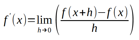
This expression serves as a general basis for linear regression when we have a dataset with various values and want the resulting affine function to have the smallest possible error. To do this, we make the value <h> approach zero. However, there is one detail here. This expression does not allow us to adjust the values of <a> and <b> in the affine function based on the resulting error. To do this, we perform several mathematical transformations and obtain the following expression.
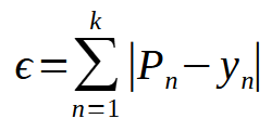
Here is the original expression for calculating the error. <P> is the value we calculate using the affine function. In turn, <y> is the estimated value or expected result. Please note that we are using an absolute value. This prevents negative and positive values from canceling each other out and thus giving the false impression that the values of <a> and <b> are correct when they are actually still incorrect. However, the expression given above does not allow us to converge quickly enough to the smallest possible error. To achieve this, we replace the absolute value with the squared error, giving us the following expression.
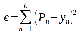
Please note that it is practically identical to the previous expression. However, using a power instead of an absolute value causes the graph of this error to change from this:
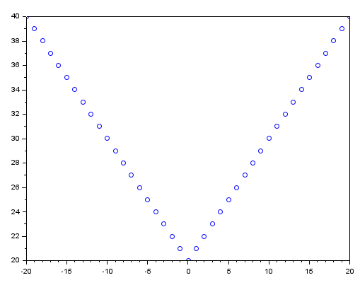
To this:
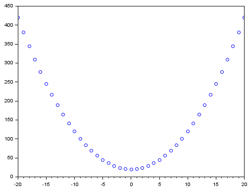
Although it may not be obvious, the difference in the rate of decrease turns out to be very significant. So significant, in fact, that if you use an even higher power, you will see the rate increase even further. You just need to make sure to use even powers, since odd powers can result in negative values. And this brings us back to the problem that we cannot simply add positive and negative values together to obtain the total error.
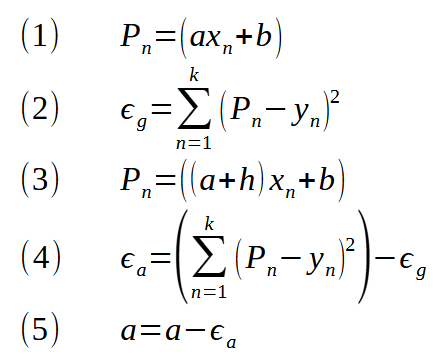
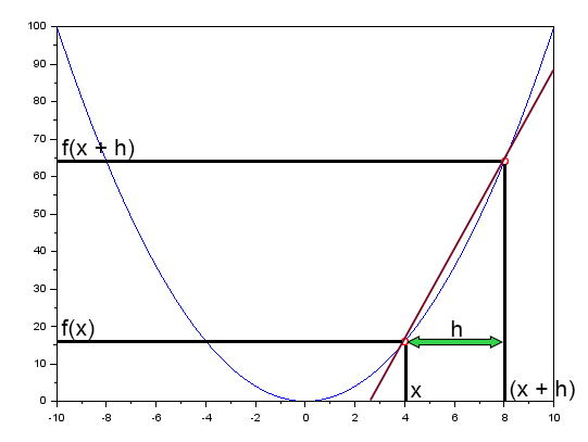
This red line is not a tangent line but a secant line, and as h approaches zero, it approaches a tangent line, becoming one when <h> equals zero. So, where does the concept of a tangent line come from? From the gradient, and nothing else. But don't worry: if you've just joined us, you'll see how it works. Returning to the topic at hand, the expression given above defines a straight line representing linear regression; therefore, we cannot represent other types of data distributions. This is why it is necessary to use what is known as an activation function. This will become clearer later. For now, it's enough to understand that without an activation function, we would be performing linear regression, which severely limits our capabilities.
However, as the number of inputs increases, the number of attempts that require us to perform steps three through five also grows very rapidly. To solve this problem, we take the expression for the least squares method and differentiate it, thereby obtaining a new expression. This expression is given below.

I know that the previous expression might seem intimidating. But it consists of all the steps necessary to determine the value required to correct the error. As you can see, a gradient is, in essence, a vector. This vector is orthogonal to the tangent line at a given point on the curve. Unlike what we used before, this gradient can use the tangent line to find the minimum error value. Thus, since we differentiate the expression for the least squares method—and this expression includes an activation function—we will also need to differentiate the activation function when calculating the gradient. For this reason, we use the derivatives of activation functions. But only during the backpropagation phase, since at this stage we are trying to ensure that the perceptron's output is treated as the input.
And one last note. You may have noticed that here I used <a> and <b> instead of the usual <w> and <b>. I did this deliberately to show that, ultimately, everything boils down to the original expression—an affine function subjected to a series of transformations until it takes gradient form.
Concluding Thoughts
In this article, you learned how and why the perceptron gradually stopped using the least squares method to correct errors in its internal constants and began using the gradient instead. We did this through a relatively smooth and simple transition, during which you began to realize that a perceptron is nothing more than a set of mathematical functions and expressions, the purpose of which is to allow us to construct a linear regression that best fits a given dataset.
So please take a close look at the code in the attached file, as it will help you understand what we'll be doing in subsequent articles. We are approaching a crucial point where you will begin to realize that certain details must be taken into account when training a perceptron system.
| MQ5 File | Description |
|---|---|
| Scripts\Example A | Basic Demonstration |
| Scripts\Example B | Basic Demonstration |
Translated from Portuguese by MetaQuotes Ltd.
Original article: https://www.mql5.com/pt/articles/13884
Warning: All rights to these materials are reserved by MetaQuotes Ltd. Copying or reprinting of these materials in whole or in part is prohibited.
This article was written by a user of the site and reflects their personal views. MetaQuotes Ltd is not responsible for the accuracy of the information presented, nor for any consequences resulting from the use of the solutions, strategies or recommendations described.