

Neural Networks in Trading: A Spatio-Temporal State Model for Financial Data Analysis (Conclusion)
 79
 4

Introduction
Work on adapting the concepts of the E-STMFlow framework has gradually reached the stage where the foundation has been laid and the mechanisms have been synchronized. Over the course of the previous two articles, we have followed a path comparable to carefully building the structural framework of a complex trading tool. First, we examined the nature of the event-driven approach, and then we recreated the key architectural components. Now, as we prepare for the final stage, it is important to pause for a moment and step back into the broader context so that our assessment of the final results is as meaningful as possible.
The idea behind E-STMFlow is the desire to work with data streams as they occur naturally. In classical computer vision, this is a stream of events from the event camera sensor array, where every minute change in brightness generates a separate signal. In the world of trading, ticks play the role of these events — tiny, real-time changes in the market that occur without a steady rhythm, without a predetermined pace, and often without any predictability. The market breathes as unevenly as the flow of events in a physical system. Sometimes fast, sometimes slow. Sometimes with sudden surges, sometimes almost imperceptibly. That is precisely why event-driven architecture, designed to analyze dynamics, has proven to be surprisingly well-suited to the nature of market data.
The E-STMFlow framework is built around a state representation that is updated with each new event. In traditional deep learning models, the data stream is divided into blocks of a fixed size. Convolutions operate on static arrays, while attention is distributed across frames prepared in advance. Here, things are different. Every event is a step. Every change involves updating internal parameters. Each new batch of data instantly affects the hidden state. In the original application, such an event was a change in a pixel's value. In our case, this refers to changes in price, volume, spread, or other features that we use to describe market momentum.
This approach is particularly valuable for financial markets, since their dynamics rarely allow for delays. Major players act in a fraction of a second. Liquidity moves in spurts. And the microstructure reacts to every movement like a mechanical pendulum that has been given a new push. Models based on candlesticks at regular time intervals inevitably smooth out these nuances and often lose the subtle structure from which trading signals emerge. The E-STMFlow architecture is precisely what allows this structure to be preserved. It does not impose artificial intervals on the market. It does not average out or interrupt the stream. Instead, it treats each new impulse as part of the overall movement and retains everything that truly matters in memory.
The essence of the original framework lies in a compact Spatio-Temporal State Space Module — a module that integrates spatial and temporal dynamics into a single state update process. In a camera, space refers to pixel coordinates; in trading, we interpret space differently — as a set of features through which the market communicates its current state. The rate of price change, the magnitude of the latest price movement, the volume reaction, and liquidity characteristics — all of these elements form a unique multidimensional space in which every tick leaves a trace. The temporal component is also important. Ticks arrive at irregular intervals, and the model must take into account not only their values but also the rhythm at which they occur.
For this reason, event-driven architecture is particularly well-suited for processing market data. It naturally filters out periods of calm. When the market is quiet, the flow of events almost disappears, and the model does not waste resources processing unnecessary information. However, when activity surges, the architecture responds immediately, updating its state at every step and forming an up-to-the-moment understanding of what is happening. This feature makes E-STMFlow an extremely attractive candidate for use in trading algorithms, where it is necessary to respond quickly to changing conditions and avoid delays.
It is also important to note the computational efficiency of the proposed approach. Unlike heavyweight transformers or deep recurrent structures, state models run quickly, consume minimal resources, and scale easily. The E-STMFlow framework allows for fine-tuning the state dimensionality, easily adapts to the characteristics of the stream being analyzed, and does not require excessive memory.
The author's visualization of the E-STMFlow framework is shown below.

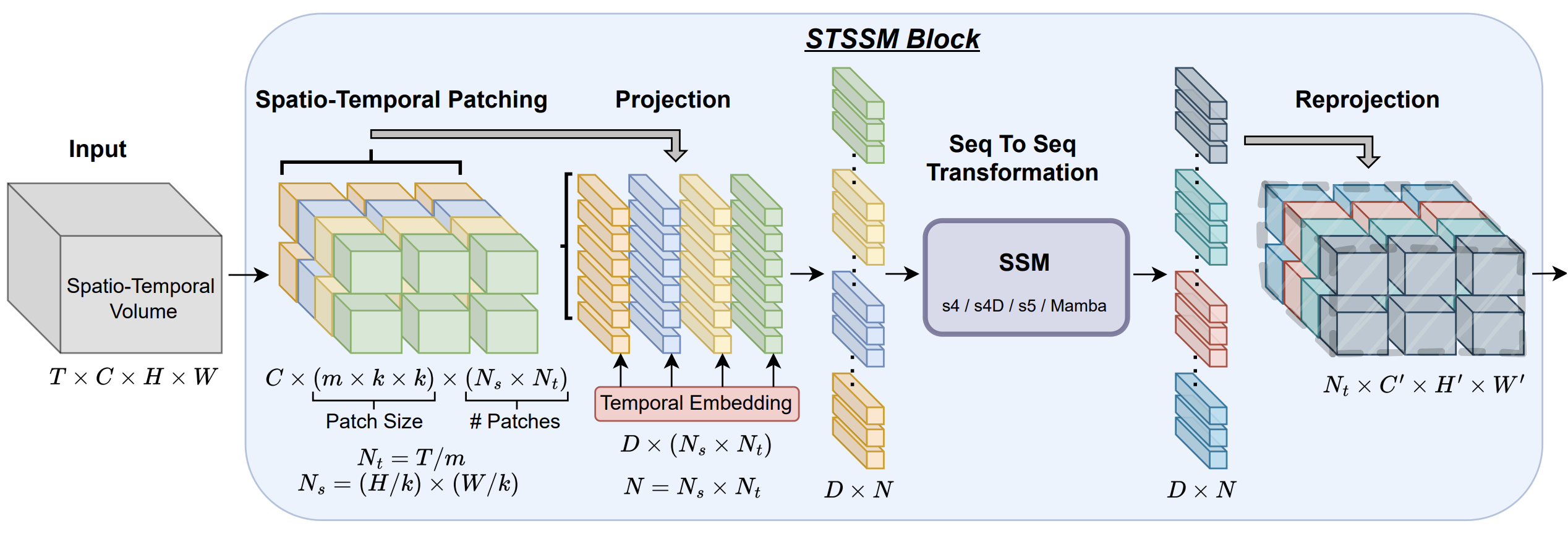
In previous articles, we have already described in detail the process of feature generation, methods for encoding events, and the mechanism for hidden state updates. We have created a structure that can receive a data stream, convert it into a compact representation, and pass it to OpenCL compute units. These blocks now contain the core processing logic. Each new event triggers a state update, and these updates gradually build an understanding of the direction and strength of the movement.
Now that we have restored the full context and regained a feel for the inner rhythm of this approach, we can move on to the final stage.
Top-level Object
Having broken down the E-STMFlow architecture into individual modules and implemented the key elements of event processing, we have now reached a stage that always feels special in engineering work. The time has come to bring all the created elements together into a single top-level object, give the system coherence, and make it function as a unified whole. This is the stage where disparate components finally begin to speak the same language, and the architecture — which until recently resembled a blueprint for a future building — gradually transforms into a fully fledged structure capable of withstanding the pressures of the real market.
It is worth noting that the developers of the E-STMFlow framework have taken a significant step forward by not only updating the encoder architecture but also offering a fresh perspective on the decoder’s design. They have, in effect, broadened the scope of traditional approaches by proposing a more robust and expressive model for working with time series. However, in our project, we deliberately left this part out of the implementation. And not because it is uninteresting or difficult. The reason runs much deeper and is linked to the practical goals we set for ourselves.
Our goal remains to create an autonomous trading robot capable not just of predicting the price at the next point in time, but of making sound trading decisions in a real, noisy, and unpredictable market. Financial charts are always bustling with activity — prices move in spurts, and liquidity fluctuates with the mood of the crowd. And even a perfect forecast can be useless if it is not backed by an understanding of market structure. Therefore, as paradoxical as it may sound, accurately predicting the next tick is not an end in itself for us. It is a useful tool, but it is not the basis for all trading behavior.
It is far more important to develop a deep, stable, and informative latent representation of the current market state — a sort of internal map that highlights key levels, impulsive moves, corrections, and hidden patterns of supply and demand. An agent with such a representation no longer acts blindly. It sees the context, not just the next number in the sequence. It understands market sentiment, not just the mechanical dynamics of candlesticks. And it is precisely the E-STMFlow encoder, with its new structure, that makes it possible to create such a rich internal state. It gives the model clarity of thought, helps it identify what is important and filter out the noise, and lays the foundation for making well-considered and consistent decisions.
That is precisely why the top-level object we are currently developing is becoming a key component of the entire implementation. It will allow individual components to be integrated into a single functional system, with the upgraded encoder serving as the heart of the system and the other modules providing flexibility and stability.
We recreate the structure of the encoder used in E-STMFlow in a new class, CNeuronESTMEncoder. It inherits from the CNeuronSpikeConvBlock block and thus gains access to all the functionality that has already proven reliable in earlier stages of development.
class CNeuronESTMEncoder   :  public CNeuronSpikeConvBlock
  {
protected:
   CLayer            cFlow;
   //---
   virtual bool      feedForward(CNeuronBaseOCL *NeuronOCL) override;
   virtual bool      calcInputGradients(CNeuronBaseOCL *NeuronOCL) override;
   virtual bool      updateInputWeights(CNeuronBaseOCL *NeuronOCL) override;

public:
                     CNeuronESTMEncoder(void) {};
                    ~CNeuronESTMEncoder(void) {};
   //---
   virtual bool      Init(uint numOutputs, uint myIndex, COpenCLMy *open_cl,
                          uint &stack_size[], uint &dimension[], uint patch_dimension,
                          uint ssm_dimension, uint &variables[],
                          ENUM_OPTIMIZATION optimization_type, uint batch);
   //---
   virtual int       Type(void)   override const   {  return defNeuronESTMEncoder;   }
   //--- methods for working with files
   virtual bool      Save(int const file_handle) override;
   virtual bool      Load(int const file_handle) override;
   //---
   virtual void      SetOpenCL(COpenCLMy *obj)   override;
   virtual void      TrainMode(bool flag) override;
   //---
   virtual bool      Clear(void) override;
   virtual bool      WeightsUpdate(CNeuronBaseOCL *source, float tau) override;
  };
The object contains the cFlow component — a separate dynamic array responsible for streaming data processing and the synchronization of computations characteristic of the E-STMFlow architecture. On the surface, the structure appears simple, but behind that simplicity lies a rather sophisticated logic, carefully crafted by the authors of the original framework.
Initializing the encoder object is the very stage at which the architecture ceases to be a diagram on paper and becomes a functioning mechanism. This is where the model takes on its dimensions, internal geometry, and sequence of computational blocks that will shape its perception of the market.
It is important to note that the E-STMFlow architecture is based on a multi-layer structure, in which each layer performs a strictly defined role. That is precisely why the initialization process is so involved. It is as if the model is being briefed before entering the real market, where there is no room for error and every failure distorts the analysis of the market situation.
bool CNeuronESTMEncoder::Init(uint numOutputs, uint myIndex, COpenCLMy *open_cl,
                              uint &stack_size[], uint &dimension[], uint patch_dimension,
                              uint ssm_dimension, uint &variables[],
                              ENUM_OPTIMIZATION optimization_type, uint batch)
  {
   uint layers = stack_size.Size();
   if(layers < 1 ||
      dimension.Size() != (layers + 1) ||
      variables.Size() != (layers + 1))
      return false;
The initialization method's algorithm begins by verifying the validity of the received parameters. It is a kind of technical check before the entire machine is started up. The stack_size, dimension, and variables arrays specify the configuration of each layer—the width and depth of the data processing streams, the internal representations, and the sizes of the hidden blocks. If at least one of these arrays has an incorrect length, further operation of the model becomes meaningless, and initialization is terminated. This approach not only ensures architectural discipline but also prevents many errors that could lead to incorrect robot behavior under real trading conditions.
After a basic check, the object relies on the functionality of the parent class, which defines the general parameters of the computational framework.
   if(!CNeuronSpikeConvBlock::Init(numOutputs, myIndex, open_cl, dimension[layers - 1],
                                   dimension[layers - 1], dimension[layers],
                                   variables[layers], 1, optimization_type, batch))
      return false;
This step can be compared to setting up the overall infrastructure. The basic settings are established. Computing resources are allocated. The model gains a foundation on which more intricate structures can be built with confidence.
Next, the internal sequence of computational blocks that make up the cFlow data processing stream begins to take shape.
   cFlow.Clear();;
   cFlow.SetOpenCL(OpenCL);
   CNeuronTransposeOCL*    transp = NULL;
   CNeuronSpikeConvBlock*  conv = NULL;
   CNeuronSpikeSTSSM*      ssm = NULL;
   uint index = 0;
Each iteration of the loop corresponds to one layer of the encoder. And in each layer, the CNeuronSpikeSTSSM module becomes a required component. This module underpins the core logic of E-STMFlow, which handles hidden states and sequences.
   for(uint i = 0; i < layers; i++)
     {
      ssm = new CNeuronSpikeSTSSM();
      if(!ssm ||
         !ssm.Init(0, index, OpenCL, stack_size[i], dimension[i], patch_dimension,
                   ssm_dimension, variables[i], optimization, iBatch) ||
         !cFlow.Add(ssm))
        {
         DeleteObj(ssm)
         return false;
        }
      index++;
This component provides resistance to market noise and allows the model to retain context, which is extremely important when analyzing financial time series. After all, the market is not a set of isolated states. Its dynamics are shaped by a chain of events, in which each subsequent price movement depends on the entire history of preceding impulses.
If the parameters of the next layer require a change in the number of variables being analyzed, a combination of transpositions and convolutional blocks is added.
      if(variables[i] != variables[i + 1])
        {
         transp = new CNeuronTransposeOCL();
         if(!transp ||
            !transp.Init(0, index, OpenCL, variables[i], dimension[i], optimization, iBatch) ||
            !cFlow.Add(transp))
           {
            DeleteObj(transp)
            return false;
           }
         index++;
         conv = new CNeuronSpikeConvBlock();
         if(!conv ||
            !conv.Init(0, index, OpenCL, variables[i], variables[i], variables[i + 1],
                       dimension[i], 1, optimization, iBatch) ||
            !cFlow.Add(conv))
           {
            DeleteObj(conv)
            return false;
           }
         index++;
         transp = new CNeuronTransposeOCL();
         if(!transp ||
            !transp.Init(0, index, OpenCL, dimension[i], variables[i + 1], optimization, iBatch) ||
            !cFlow.Add(transp))
           {
            DeleteObj(transp)
            return false;
           }
         index++;
        }
This may seem like a technical detail, but it actually serves as a subtle adjustment to the architecture to accommodate the changing sizes of latent representations. This mechanism is similar to adjusting trading instruments to suit a specific market regime. The model modifies its internal structure to maintain consistency in computations and prevent the loss of important information at the layer boundaries.
After processing each level, a convolutional block is added to the data stream to prepare the data for the next layer.
      if(i == (layers - 1))
         break;
      conv = new CNeuronSpikeConvBlock();
      if(!conv ||
         !conv.Init(0, index, OpenCL, dimension[i], dimension[i], dimension[i + 1],
                    variables[i + 1], 1, optimization, iBatch) ||
         !cFlow.Add(conv))
        {
         DeleteObj(conv)
         return false;
        }
      index++;
     }
//---
   return true;
  }
These blocks enhance the model's ability to identify key elements of market structure, thereby stabilizing the flow of information to deeper layers of the network.
Ending at the final layer, the loop forms a coherent, sequential computational path that data will follow during training and inference.
As a result, the encoder ends up with a streamlined, well-organized processing pipeline, where each module is in its proper place and every transformation is precisely calculated. This initialization may seem overly detailed, but it is entirely justified when working with real financial data. The market is unforgiving of ill-defined models — even the slightest error in the architecture will result in an incorrect price assessment, and thus in incorrect trading decisions. Therefore, the strict sequence of steps in the initialization method is not a mere formality, but a guarantee that the model will operate reliably and consistently, just as intended.
The forward pass algorithm takes on an almost linear form thanks to the dynamic array cFlow, which links all elements of the architecture in a strict sequence. This approach makes the computational path transparent and predictable. Data moves from one block to another without branching, as if traveling down a corridor where every step is predetermined by the architecture. In the context of financial markets, this is particularly important because the sequence of transformations must be stable and the model must be reproducible. Any uncertainty in the structure can lead to undesirable artifacts in the processing of price data.
bool CNeuronESTMEncoder::feedForward(CNeuronBaseOCL *NeuronOCL)
  {
   CNeuronBaseOCL* prev = NeuronOCL;
   CNeuronBaseOCL* curr = NULL;
   for(int i = 0; i < cFlow.Total(); i++)
     {
      curr = cFlow[i];
      if(!curr ||
         !curr.FeedForward(prev))
         return false;
Within the feedForward method, we begin by passing the data to be analyzed to the first module and then sequentially pass control to each object stored in cFlow. Each module receives the result from the previous one and performs its part of the calculations, forming an increasingly meaningful latent representation.
This approach is similar to a step-by-step analysis of the market situation. First, we assess the local price structure; then we relate it to the context; and finally, we take broader factors into account. In this sense, linear processing provides a natural framework for identifying patterns in price movements.
However, the architecture is linear only at first glance. In fact, the behavior of the STSSM blocks plays a key role here. Each time the model passes through the CNeuronSpikeSTSSM module, we apply an additional transformation to its results — a residual connection operation that routes part of the previous signal directly to the output of the current block.
      if(curr.Type() == defNeuronSpikeSTSSM)
         if(!SumAndNormilize(prev.getOutput(), curr.getOutput(), curr.getOutput(), 1, false, 0, 0, 0, 1))
            return false;
      prev = curr;
     }
This mechanism reflects the core idea of E-STMFlow, on which the entire algorithm is based. The SSM component predicts the relative change in the stream, while the residual connection keeps the model anchored to the original values. As a result, the encoder ceases to be a predictor of absolute values and becomes a flexible mechanism that tracks the dynamics of the sequence's state.
In the context of financial time series, this approach is more than justified. The market rarely moves in a straight line and almost never reveals its direction in advance. It is more important to be able to detect changes: accelerations, decelerations, shifts in rhythm, and changes in volatility. A latent representation based solely on absolute values quickly loses its sensitivity to these nuances. However, a system that operates on relative changes and maintains a connection to its previous state gains an advantage. It can adapt to market regimes without losing context. The residual connections following the SSM blocks act as a sort of anchor, keeping the model in a stable state and preventing it from deviating too far or drifting into the realm of overly complex transformations.
That is precisely why the forward pass method is compact, but by no means primitive. It consists of a carefully calibrated combination of linear architecture and dynamic adjustments built directly into the logic of the STSSM blocks. This structure allows the model to generate a rich, robust, and informative latent space that can be used as a basis for making trading decisions. For the future trading agent, this means clearer and more stable market analysis. This, in turn, means better-founded behavior in the face of real-world price fluctuations.
After all iterations of the loop have been completed, control is passed to the method of the same name in the parent class.
   return CNeuronSpikeConvBlock::feedForward(prev);
  }
This step plays an important role in the overall logic of the encoder. As the data stream passes through a sequence of internal cFlow modules, we transform the original signal step by step, enriching it with local structures, the dynamics of change, and adjustments specified by the SSM blocks. But it is the final call to the base class method that completes this process and transforms all the accumulated information into a coherent, neatly organized view of the market situation.
This final stage can be compared to how a trader, after a series of observations and interim assessments, finally organizes their thoughts and formulates a specific conclusion. Internal modules provide us with rough sketches — the structures of local patterns, the pace of change, and contextual connections. The parent class's feedForward method, in turn, acts as the final editor. It takes the result from the last block in the chain, applies the necessary transformations, and provides the user with a stabilized, consistent representation that can be passed on to the next stage of processing.
It is also important to note that this final format is determined in advance by the model's configuration. The user specifies the parameters, selects the number of features and the dimensionality of the output space — and the parent class generates the result in exactly this format. This makes the architecture flexible. A single encoder can be adapted to different market analysis frameworks, ranging from compact latent representations for a trading agent to large-scale multidimensional signals for complex analytical systems. In effect, the data undergoes final packaging tailored to the specific task and the requirements of the trading strategy.
The backward pass phase is like a moment of reflection after a trading session. This is when an experienced trader sits down with tables and charts to figure out where their decisions aligned with the market and where they missed the mark. In the context of our encoder, the calcInputGradients method serves precisely this purpose. It allows the model to evaluate its predictions, identify errors, and distribute them across all internal components, turning every deviation into a learning tool.
bool CNeuronESTMEncoder::calcInputGradients(CNeuronBaseOCL *NeuronOCL)
  {
   if(!NeuronOCL)
      return false;
The process begins by verifying that the pointer to the source data object is valid. This ensures that we have the correct data to work with. Next, the method of the same name in the parent class is called, which passes the error gradients to the last element in the cFlow chain.
   if(!CNeuronSpikeConvBlock::calcInputGradients(cFlow[-1]))
      return false;
This step can be thought of as locking in the final result; it serves as the starting point for all subsequent adjustments.
Next, the process moves backward along the chain, starting with the second-to-last element and proceeding toward the first. At each step, the CalcHiddenGradients method is called for the current block, allowing the local error to be computed based on information received from the next level.
   CNeuronBaseOCL* next = cFlow[-1];
   CNeuronBaseOCL* curr = NULL;
   for(int i = cFlow.Total() - 2; i >= 0; i--)
     {
      curr = cFlow[i];
      if(!curr ||
         !curr.CalcHiddenGradients(next))
         return false;
This algorithm creates a chain of cause and effect. If an error occurs at a higher level, each lower-level block assumes its share of responsibility and adjusts its own parameters. This approach ensures that each part of the model knows what it is responsible for and does not overload its neighbors with unnecessary adjustments.
Special attention is given to STSSM blocks. In the forward pass, we added residual connections, so in the backward pass, the gradients must be carefully adjusted to account for these connections.
      if(next.Type() == defNeuronSpikeSTSSM)
        {
         if(curr.Activation() != None)
           {
            if(!DeActivation(curr.getOutput(), next.getPrevOutput(), next.getGradient(), curr.Activation()) ||
               !SumAndNormilize(next.getPrevOutput(), curr.getGradient(), curr.getGradient(), 1, false, 0, 0, 0, 1))
               return false;
           }
         else
            if(!SumAndNormilize(next.getGradient(), curr.getGradient(), curr.getGradient(), 1, false, 0, 0, 0, 1))
               return false;
        }
      next = curr;
     }
It is worth noting here that the flow of operations depends on whether the layer preceding the STSSM block has an activation function. If an activation function is present, the DeActivation method is used first. It allows the gradients along the residual connection path to be adjusted with respect to the derivative of the activation function, and only then are the error gradients obtained from the two information streams summed. If there is no activation function, this unnecessary operation is omitted.
Thanks to this design, STSSM blocks are trained not on absolute values but on relative changes in the data stream, which is ideally suited to analyzing financial time series. After all, it is important to capture the dynamics rather than record static levels.
After we have iterated through the entire cFlow array, the error gradients are passed down to the raw data level.
//---
   if(!NeuronOCL.CalcHiddenGradients(next))
      return false;
   if(next.Type() == defNeuronSpikeSTSSM)
     {
      if(NeuronOCL.Activation() != None)
        {
         if(!DeActivation(NeuronOCL.getOutput(), next.getPrevOutput(), next.getGradient(),
                                                                 NeuronOCL.Activation()) ||
            !SumAndNormilize(next.getPrevOutput(), NeuronOCL.getGradient(),
                                             NeuronOCL.getGradient(), 1, false, 0, 0, 0, 1))
            return false;
        }
      else
         if(!SumAndNormilize(next.getGradient(), NeuronOCL.getGradient(),
                                             NeuronOCL.getGradient(), 1, false, 0, 0, 0, 1))
            return false;
     }
//---
   return true;
  }
A check is also made here to determine whether an activation function is present. And, if necessary, the same logic for adjusting gradients is applied, taking into account the residual connection. This allows the entire backward pass to be completed cleanly, without leaving any gaps in the distribution of errors across the layers.
As a result, the entire method generates a structured gradient map, and each block understands how its weight influenced the final result and in which direction it needs to be adjusted.
This is particularly valuable for financial analysis. The model doesn't simply repeat past movements; it learns to identify key dynamic patterns, recognize hidden signals, and adapt to changing market conditions. This approach ensures the trading agent’s robustness, accuracy, and operational stability even amid high volatility and unpredictable market swings, turning each training cycle into a means of improving the model’s proficiency.
Taken as a whole, the CNeuronESTMEncoder class serves as the very point of convergence where engineering logic meets financial practice. It prepares data for subsequent modules, forms the core of market understanding, and ensures the cohesion of the entire architecture. And the more accurately, reliably, and cleanly we implement it, the more confident our agent will feel. The complete code for this class and all of its methods is provided in the attachment.
Model Architecture
As previously mentioned, in this project we are developing a full-fledged trading system capable of independently analyzing the market, making decisions, and executing trades. The model's architecture is generally based on proven solutions from previous work, which has made it possible to retain reliable signal processing and learning algorithms. Significant changes were made only to the environment encoder — this is where the top-level object CNeuronESTMEncoder was introduced, becoming the core component for generating the market's latent representation.
//--- Layer 4
   if(!(descr = new CLayerDescription()))
      return false;
   descr.type = defNeuronESTMEncoder;
     {
      uint temp[] = {prev_out,                  // Channels In
                     16,
                     32,
                     64,
                     64                         // Channels Out
                    };
      if(ArrayCopy(descr.windows, temp) < (int)temp.Size())
         return false;
     }
     {
      uint temp[] = {prev_count,                // Units In
                     12,
                     24,
                     12,
                     12                         // Units Out
                    };
      if(ArrayCopy(descr.units, temp) < (int)temp.Size())
         return false;
     }
A new layer is created using a CLayerDescription object, which specifies all of the layer's parameters. For each level, we specify the number of input and output channels, the number of elements in the sequence, the stack sizes, and other characteristics.
Special attention should be paid to stack sizes at each level of data analysis. In the original framework, the authors propose progressively reducing the temporal dimension until it reaches 1 at the encoder's final output. We follow this logic, gradually reducing the stack size at each layer, but retain a short temporal history at the final level. This allows us to retain some information about recent market movements, which is critical for accurately assessing trends and short-term price fluctuations. This approach combines the benefits of the original methodology with the requirements of our task. The model receives a compact yet informative representation of time series that supports consistent trading decisions.
     {   // Stack size
      uint temp[] = {48,
                     24,
                     12,
                     4
                    };
      if(ArrayCopy(descr.heads, temp) < (int)temp.Size())
         return false;
     }
   descr.window=16;
   descr.window_out=64;
   descr.optimization = ADAM;
   descr.batch = BatchSize;
   if(!encoder.Add(descr))
     {
      delete descr;
      return false;
     }
Particular attention is paid to the model parameter optimization method (ADAM) and the batch size (BatchSize). These parameters ensure stable training on historical data.
This approach offers us several advantages. First, the architecture remains clear and transparent — each parameter is easy to track and adjust as needed. Second, flexibility is maintained — modifying individual layers or adding new components does not require sweeping changes. Third, the system is ready to adapt to different market conditions, as the new encoder fits seamlessly into the model’s existing structure, providing an enriched and informative latent representation of the market state.
Taken together, this makes it possible to build a trading agent capable of operating autonomously and consistently, based on structured signals derived from market data. The complete code defining the architecture is available in the attachment, allowing you to reproduce and extend the implementation without compromising the model's integrity.
Testing
Once the model architectures have been defined, we move on to the final stage — training and testing. As before, this process consists of two stages, and each plays a key role in shaping a comprehensive trading strategy for the agent.
The first stage of training is based on historical data and is similar to a beginner trader's practice session on a major exchange. Imagine the EURUSD chart from January 2024 to June 2025 as a canvas full of hidden patterns. Like an attentive student, the model scrutinizes every candlestick, tracks volume, analyzes market reactions to indicators, and identifies patterns. Our implementation of the E-STMFlow framework's encoder makes it possible to detect the slightest price fluctuations while also identifying broader trends. It generates an informative state for the Actor and the Critic, combines features of different scales, and learns alongside the model. With each new step, the model gradually becomes a confident trader capable of making independent decisions.
The next stage — online training in the MetaTrader 5 Strategy Tester — is no longer just a rehearsal, but intensive skills practice. There is no convenient historical data here; each candlestick represents a live pulse of the real market. The model reacts instantly, evaluates noise fluctuations, adapts to sudden spikes, and adjusts its actions during periods of low liquidity. CNeuronESTMEncoder synchronizes the operation of all blocks, integrates features across different scales, and continues learning alongside the model, resulting in flexible and stable behavior.
The final skills assessment uses data from July through October 2025. There are no clues here, and no way to rely on the past — only the market and the model's decisions. Every move hones the ability to combine features of different scales, anticipate market reactions, and act with precision. The test results demonstrate how the implemented solution transforms a complex architecture into a cohesive, adaptive, and efficient trading system.


The test results show a smooth, balanced capital trajectory with moderate volatility. The balance and equity are moving in tandem, which indicates the stability of the strategy's performance and the proper functioning of the algorithms that process market information.
The first two months of the testing period were characterized by sideways movement, with slight fluctuations around the initial deposit level. This reflects the absence of a clear trend advantage in the market segment under consideration and indicates that the robot does not force trades without sufficient signals. It is only in the second half of the period that steady capital growth is observed. The balance curve reaches approximately 103.8 USD and remains in this range until the end of the test, demonstrating the strategy's ability to identify and capitalize on favorable market opportunities.
The maximum balance drawdown was 4.02%, and the maximum equity drawdown was 5.48%. These indicators reflect the system's conservative risk profile and stability. The strategy avoids deep drawdowns, maintaining a margin of safety and ensuring prudent capital management, which is especially important with a small initial deposit.
Net profit reached 3.29%, with a profit factor of 1.35. This means that every USD of risk yields a profit of 1.35 USD. This value is sufficient for the initial stage of algorithm development, although it indicates potential for further optimization of entries and exits to improve overall efficiency.
The expected payoff per trade is 0.13 based on 26 completed trades, which confirms a moderately positive shift in the distribution of results. The recovery factor is 0.59, indicating a moderate rate of recovery to the previous level after drawdowns. The low standard error of the linear regression (0.63) confirms that the equity curve is smooth, with no sharp noise spikes.
The trade mix is balanced: of the 26 trades, 53.85% were profitable. Long and short positions had roughly similar success rates. The maximum profit per trade reached 3.00 USD, and the maximum loss was 1.46 USD. This results in a moderately favorable win-to-loss ratio.
Overall, testing confirms that the robot’s logic, implemented using E-STMFlow, delivers modest but positive capital growth, minimal drawdowns, a predictable risk distribution, and stable performance. Despite the modest absolute profit, the shape of the curve, the quality of the risk profile, and the consistency of the metrics indicate that the strategy has high potential. Key areas for future work include improving the accuracy of entries, locally optimizing trend filters, and adaptively calibrating stop parameters to increase expected returns without significantly increasing risk.
Conclusion
Our work demonstrates the practical effectiveness of the E-STMFlow framework in building an autonomous trading system. The implementation of the top-level object CNeuronESTMEncoder made it possible to integrate the individual components of the architecture into a single, cohesive structure, ensuring an accurate and informative representation of the market state. Successive reductions in stack sizes and the introduction of a short temporal history made it possible to preserve critical information about recent price movements, which improved the robustness of trading decisions.
Training and testing the model on historical data confirmed the strategy's stability, moderate capital growth, low drawdowns, and predictable risk distribution. The results showed that the robot is capable of adapting to market volatility, adjusting its actions amid noise-driven fluctuations, and maintaining a balanced ratio of wins to losses.
The proposed solution shows great potential for building autonomous trading agents. The combination of modular architecture, sophisticated processing of features at different scales, and trainable connections between components creates the foundation for a reliable and adaptive system. The strategy can be further developed by optimizing entries and adaptively adjusting filters and stop parameters. These improvements would increase profitability without significantly increasing risk, transforming the prototype into a fully fledged tool for professional traders.
Links
- Spatio-Temporal State Space Model for Efficient Event-Based Optical Flow
- Other articles in this series
Software used in this article
| # | Name | Type | Description |
|---|---|---|---|
| 1 | Study.mq5 | Expert Advisor | Expert Advisor for offline model training |
| 2 | StudyOnline.mq5 | Expert Advisor | Expert Advisor for online model training |
| 3 | Test.mq5 | Expert Advisor | Expert Advisor for model testing |
| 4 | Trajectory.mqh | Class library | Structure describing the system state and model architectures |
| 5 | NeuroNet.mqh | Class library | Class library for building a neural network |
| 6 | NeuroNet.cl | Library | Code library for an OpenCL program |
Translated from Russian by MetaQuotes Ltd.
Original article: https://www.mql5.com/ru/articles/20477
Warning: All rights to these materials are reserved by MetaQuotes Ltd. Copying or reprinting of these materials in whole or in part is prohibited.
This article was written by a user of the site and reflects their personal views. MetaQuotes Ltd is not responsible for the accuracy of the information presented, nor for any consequences resulting from the use of the solutions, strategies or recommendations described.



Training for 3 or even 30 epochs is very little. In ‘...\Experts\NeuroNet_DNG\NeuroNet.mqh’, the learning rate is set to
Using a VAE, unlike other types of neural layers, allows you to learn the boundaries of the distribution of values, rather than just the mean.
And yes, E-STMFlow does not support either VAEs or the Actor-Critic model as such.
Good evening,
Training for 3 or even 30 epochs is far too little. In ‘...\Experts\NeuroNet_DNG\NeuroNet.mqh’, the learning rate is set to
. Unlike other types of neural layers, using a VAE allows you to learn the boundaries of the distribution of values, rather than just the mean.
And yes, E-STMFlow does not support either VAEs or the Actor-Critic model as such.
Main performance issues:
1.Sequential processing on the CPU instead of batching on the GPU
. The code processes each position in turn within a loop. For each bar, the following is executed:- This
amounts to2. Multiple CPU-GPU synchronisations
EachfeedForward/backProp call requires data transfer between the CPU and GPU, creating a huge overhead.3. Inefficient use of BatchSize
. BatchSize is set to 1e4, but the code processes one example at a time instead of in batches.As a result, I’ve decided to try porting your idea to Python, using the source code from the original article as a basis and adapting it according to your approach. Let’s see how it turns out. Or perhaps you could suggest a performance solution for MQL5? Or at least point me in the right direction?
I’m really pleased to hear your feedback. I suppose that even 100 epochs wouldn’t be enough for high-quality training. But the funny thing is that even on a rented server with a good GPU, the training process is extremely slow. Neither the CPU nor the graphics card is utilised to full capacity, averaging only about 10 per cent. To run 1,000+ epochs, I’ll have to keep the server running for at least two weeks... The problem is that the code runssequentially on the CPU, despite OpenCL being initialised.
Main performance issues:
1.Sequential processing on the CPU instead of batching on
the GPU. The code processes each position one by one in a loop. For each bar, the following is executed:- This
amounts to2. Multiple
CPU–GPUsynchronisations:
EachfeedForward/backPropcall requires data transfer between the CPU and GPU, creating a huge overhead.3. Inefficient use
of BatchSize: BatchSize is set to 1e4, but the code processes one example at a time instead of in batches.As a result, I’ve decided to try porting your idea to Python, using the source code from the original article as a basis and adapting it according to your approach. Let’s see how it turns out. Or perhaps you could suggest a performance solution for MQL5? Or at least point me in the right direction?