Neural Networks in Practice: The Gradient

Introduction

In the previous article, we implemented an application designed to study the behavior of derivatives and activation functions. Understanding what was explained there will help you understand what we'll be covering here.

In this article, I will try to explain how and why the gradient came to be used in training a perceptron network. At first, the mathematics behind the gradient may seem a bit confusing and difficult to understand. However, I'll use a much simpler method so that you can understand once and for all how a gradient works in practice. So, let's set aside everything that distracts us and focus on what will be explained in this article, since understanding how the gradient works is essential for understanding other topics we'll cover later.

Why a gradient?

Since I don't know how familiar each of you is with the mathematical aspects, I'll try to explain this point slowly and clearly. The actual programming is the easy part. It's hard to understand—and, above all, to explain—the mathematical part. Many might say that the math—which, in essence, constitutes the theoretical part of what we're going to implement—can be ignored altogether, and we can move straight to the code.

Personally, I think that if I show you only the code, you'll eventually hit a dead end. I've already mentioned this, and I'll say it again: THERE IS NO STANDARD MODEL FOR CREATING NEURAL NETWORKS. Every case is unique. Understanding how each part of a perceptron works is essential to understanding the perceptron as a whole and making the necessary connections when deciding which operations to use. Don't make the mistake of thinking that a particular implementation can solve any problem. Even if you try to train it to create a model that represents a specific dataset, you won't always be able to use the same implementation with a completely different dataset, since it will rarely work correctly.

I've already touched on the topic of the gradient in another article. However, I believe that certain aspects were explained very poorly there. Perhaps that is precisely why so many people are confused about this issue. I'll explain this much more simply here, because we'll soon be moving on to a much more complex topic. For now, we won't be adding activation functions to the C_Neuron class. The thing is, I don't want to complicate things prematurely and unnecessarily.

So, the gradient is a much simpler and more convenient way to represent the derivative. Or, more precisely, a way to actually use the tangent line when we're working with multiple variables. Thus, in many cases, we can use a more efficient computation method to achieve convergence.

First and foremost, it is important to understand that any gradient is, in essence, a vector. And what does that mean in practice? The first implication is that, as a vector, it points in a specific direction. In this case, it points in the direction of steepest increase. However, if we use it in the opposite direction, we can move toward the smallest increase or, in our case, toward a lower value of the loss function. That is precisely why, when moving in the direction opposite to the gradient, we refer to it as gradient descent.

The second point—and this is where many people get confused—is that the gradient is an orthogonal vector. For this reason, it is literally perpendicular to another line that passes through the vector's initial point. It is precisely this line that is the tangent line. Please keep this in mind, because it will be important later. This differs from what happens in the least squares method, where a secant line is actually constructed. Many people mistakenly claim that a perceptron uses a tangent line. However, if we analyze the calculations being performed, it becomes clear that we are actually dealing with a secant line. Therefore, be careful when specifying which type of line you are using in trigonometric calculations. There are other aspects related to vectors, but for the purposes of these articles, what we have just mentioned is more than enough to explain the entire subject.

Therefore, since the gradient is a vector, it is much more convenient to work with it in many situations. Here, however, we will focus on the most basic aspect—at least for now. Otherwise, we'll start discussing topics unrelated to the main issue.

So, the code we're going to modify—or, more precisely, enhance with new functionality—was discussed in the article. There, we simply added the code for the least squares method. The function shown below is used for this.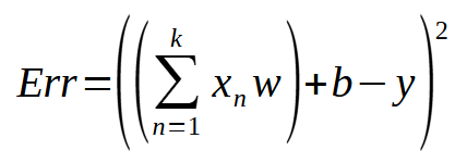

This is the expression we use to calculate the error for each row of training data using the least squares method. Here, < t > denotes the number of inputs to the perceptron. < w > denotes each of the weights. < b > denotes the bias, and < y > denotes the estimated value obtained during the training process. All right. The question is how we can transform this expression into a gradient. The answer is this: by using the mathematical concept of derivatives.

If you look at this mathematical expression and have even a basic understanding of mathematics, you will notice that there is another, very similar expression known in differentiation as the chain rule. This expression is given below.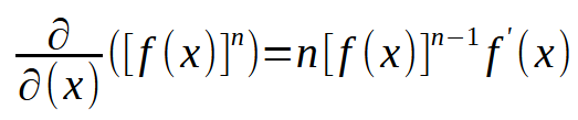

Looking at this expression, you probably shudder a little because it seems quite complicated. Actually, it's pretty simple and clearly shows what we need to do. Here, x represents the expression we want to differentiate, and n is the exponent, which in this case is equal to two. Therefore, the number 2 becomes a multiplier. The new exponent is equal to the previous one minus one. And this new expression is multiplied by the first derivative of the original expression. It's that simple. However, since our original expression contains at least two variables—weight and bias—we will write a new expression using gradient notation. Thus, the expression takes the following form.

"No, that doesn't help. These expressions still look pretty intimidating." Well, I'm sorry, but we won't be able to move forward until we work through some difficulties. Anyone who truly wants to learn something must overcome certain challenges. Now listen carefully. There is a derivative at the end of this expression. This is called a partial derivative. Standard mathematical notation differs somewhat from the notation I use here. But the point is not to present the expression in a mathematically flawless form. The point is to show how we obtain the gradient that we need to implement in code. This partial derivative is the result of three other derivatives. We can simplify the expression above even further. The following image shows how to do this.

After a few transformations to simplify the expression, we will obtain the expression shown below. That is, of course, assuming I didn't make any mistakes in the differentiation.

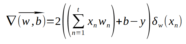
That is exactly the expression we'll have to use. It may not be written entirely correctly from a mathematical standpoint. But I'm not here to explain math or tell you how to write mathematical expressions. I'm here to show you how to convert mathematical expressions into usable code. And although the expression given above is not entirely correct in terms of mathematical notation, it is quite sufficient to explain exactly what we need to implement.

This is because here I demonstrate both how to calculate the bias and how to calculate the weights when a perceptron has multiple inputs. It might be better to write most of this expression in matrix form and use a slightly different notation for the partial derivative at the end. However, as I just mentioned, I'm not particularly concerned with absolute rigor in mathematical notation, as long as the code is written correctly. After all, we don't want something that behaves strangely or unpredictably.

All right, we've reached a crucial point. Now we can take a quick look at the resulting C_Neuron class, with its gradient correctly computed and ready to use. The code below shows what the previous expression looks like when implemented in code. Of course, we're showing the complete code here. But don't worry—I'll focus my explanation only on the part related to the gradient. We'll discuss this in the next section.

//+------------------------------------------------------------------+
#property copyright "Daniel Jose"
//+------------------------------------------------------------------+
#define macroRandom (rand() / (double)SHORT_MAX)
//+------------------------------------------------------------------+
class C_Neuron
{
    private:
//+------------------------------------------------------------------+
        struct  stInfos
        {
            bool    IsFx;
            uint    nInputs;
            double  Bias,
                    Weight[];
        }m_Infos;
//+------------------------------------------------------------------+
        struct stErr
        {
            double  weight[],
                    eMaxWeight,
                    bias;
        }m_Error;
//+------------------------------------------------------------------+
        inline double Cost_FX(const double &train[])
        {
            double x, err;

            err = 0;
            for (uint c0 = 0; c0 < train.Size(); c0++)
            {
                x = 0;
                for(uint c1 = 0; c1 < m_Infos.nInputs; c1++, c0++)
                   x += (train[c0] * m_Infos.Weight[c1]);
                err += MathPow((x + m_Infos.Bias) - train[c0], 2);
            }

            return err;
        }
//+------------------------------------------------------------------+
        inline double Learning_FX(const double &train[], const double epsilon,  const double LearningRate, const ulong limit)
        {
            double  err,
                    memT,
                    err_w[];
            ulong   count;
 
            Print("Cost being calculated by the Minimum Square...");
            ArrayResize(err_w, m_Infos.nInputs);
            for (count = 0; (count < limit) && ((err = Cost_FX(train)) > epsilon); count++)
            {
                for (uint c = 0, m = m_Infos.Weight.Size(); c < m; c++)
                {
                    memT = m_Infos.Weight[c];
                    m_Infos.Weight[c] += LearningRate;
                    err_w[c] = Cost_FX(train) - err;
                    m_Infos.Weight[c] = memT;
                }
                memT = m_Infos.Bias;
                m_Infos.Bias += LearningRate;
                m_Infos.Bias = memT - (Cost_FX(train) - err);
                for (uint c = 0, m = m_Infos.Weight.Size(); c < m; c++)
                    m_Infos.Weight[c] -= err_w[c];
            }
            PrintFormat("Total interactions: %I64u", count);
            ArrayFree(err_w);
 
            return err;
        }
//+------------------------------------------------------------------+
        inline double Cost_DX(const double &train[])
        {
            double  x1, t;

            ZeroMemory(m_Error);
            for (uint c0 = 0, cw = 0; c0 < train.Size(); c0++, cw = c0)
            {
                x1 = 0;
                for(uint c1 = 0; c1 < m_Infos.nInputs; c1++, c0++)
                   x1 += (train[c0] * m_Infos.Weight[c1]);
                t = 2 * ((x1 + m_Infos.Bias) - train[c0]);
                for(uint c1 = 0; c1 < m_Infos.nInputs; c1++, cw++)
                {
                    m_Error.weight[c1] += (t * train[cw]);
                    m_Error.eMaxWeight = (MathAbs(m_Error.weight[c1]) >  MathAbs(m_Error.eMaxWeight) ? m_Error.weight[c1] : m_Error.eMaxWeight);
                }
                m_Error.bias += t;
            }
            return (MathAbs(m_Error.bias) > MathAbs(m_Error.eMaxWeight) ? m_Error.bias : m_Error.eMaxWeight);
        }
//+------------------------------------------------------------------+
        inline double Learning_DX(const double &train[], const double epsilon, const double LearningRate, const ulong limit)
        {
            ulong   count;
            double  eRet;
            
            Print("Cost being calculated by the Gradient...");
            for (count = 0; (count < limit) && (MathAbs(eRet = Cost_DX(train)) > epsilon); count++)
            {
                m_Infos.Bias -= (m_Error.bias * LearningRate);
                for (uint c = 0, m = m_Infos.Weight.Size(); c < m; c++)
                    m_Infos.Weight[c] -= (m_Error.weight[c] * LearningRate);
            }
            PrintFormat("Total interactions: %I64u", count);

            return eRet;
        }
//+------------------------------------------------------------------+
    public :
//+------------------------------------------------------------------+
        C_Neuron(const uint nInputs = 1, const bool isFx = false, double H = 1.0, double L = 0.0)
        {
            MathSrand(512);
            ZeroMemory(m_Infos);
            m_Infos.IsFx = isFx;
            m_Infos.Bias = (double)macroRandom;
            ArrayResize(m_Infos.Weight, m_Infos.nInputs = nInputs);
            ArrayResize(m_Error.weight, m_Infos.nInputs);
            for(uint c = 0; c < m_Infos.nInputs; c++)
                m_Infos.Weight[c] = ((double)macroRandom * (H - L)) + L;
        }
//+------------------------------------------------------------------+
        ~C_Neuron()
        {
            ArrayFree(m_Infos.Weight);
            ArrayFree(m_Error.weight);
        }
//+------------------------------------------------------------------+
        void View_Variables(void)
        {
            Print("Bias: ", m_Infos.Bias);
            for (uint c = 0, m = m_Infos.Weight.Size(); c < m; c++)
                PrintFormat("Weight[%d]: %.16f", c, m_Infos.Weight[c]);
        }
//+------------------------------------------------------------------+
        inline double Learning(const double &train[], const double epsilon = 1e-3, const double LearningRate = 1e-2, const ulong limit = ULONG_MAX)
        {
           return (m_Infos.IsFx ? Learning_FX(train, epsilon, LearningRate, limit) : Learning_DX(train, epsilon, LearningRate, limit));
        }
 //+------------------------------------------------------------------+
};
//+------------------------------------------------------------------+
#undef macroRandom
//+------------------------------------------------------------------+

Notice how different this code is from the code we saw in the article where it first appeared. The fact is that we now have a completely new implementation, the main goal of which is to implement the gradient while preserving the loss function based on the least squares method. Either option can be selected for the perceptron when the constructor runs. Keep in mind that once a selection has been made in the constructor, you will no longer need to tell the perceptron whether to use the gradient or the least squares method to compute the loss function.

Please also note that a new variable has been added to the Learning function. This new variable will come in handy later. In the meantime, let's see if this perceptron is working correctly. To do this, we use the script code shown below.

//+------------------------------------------------------------------+
#property copyright "Daniel Jose"
//+------------------------------------------------------------------+
#include <Neural Network\C_Neuron.mqh>
//+------------------------------------------------------------------+
double Train[] {
                0, 0,
                1, 2,
                2, 4,
                3, 6,
                4, 8
               };
//+------------------------------------------------------------------+
void OnStart()
{
    C_Neuron *neuron;

    Print("************************************");
    Print("Simple Neuron in Class...");

    neuron = new C_Neuron(1);

    (*neuron).View_Variables();
    Print("********** RESULT *************");
    Print("Error: ", (*neuron).Learning(Train));
    (*neuron).View_Variables();

    delete neuron;
}
//+------------------------------------------------------------------+

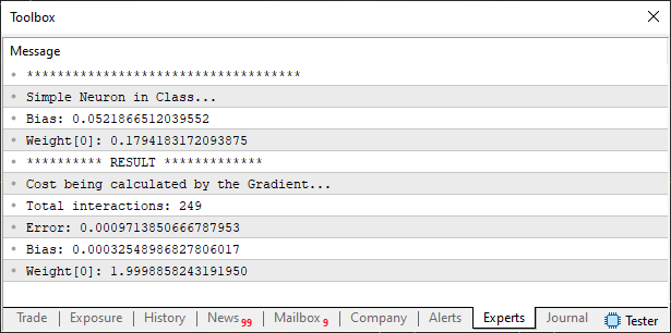
When you run this script in MetaTrader 5, you'll see exactly what's shown in the following image:

Note that we are using the gradient and that the result is very close to the expected value. However, in this test, we use only one input to the perceptron. What would happen if we modified the training code to use more inputs? What would the code look like then? To answer this question, just take a look at the code below.

//+------------------------------------------------------------------+
#property copyright "Daniel Jose"
//+------------------------------------------------------------------+
#include <Neural Network\C_Neuron.mqh>
//+------------------------------------------------------------------+
double Train[] {
                  1,    3,  10.35,
                1.5,  3.25, 11.7875,
                1.75, 3.94, 13.721,
                2.85, 3.46, 14.669
               };
//+------------------------------------------------------------------+
void OnStart()
{
    C_Neuron *neuron;

    Print("************************************");
    Print("Simple Neuron in Class...");

    neuron = new C_Neuron(2);

    (*neuron).View_Variables();
    Print("********** RESULT *************");
    Print("Error: ", (*neuron).Learning(Train));
    (*neuron).View_Variables();

    delete neuron;
}
//+------------------------------------------------------------------+

Now we have two inputs so that the neuron can arrive at a solution. The result that will appear in MetaTrader 5 is shown in the following image.

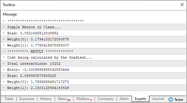
And, just as before, the result turns out to be extremely close to the correct values. This indicates that our gradient is working correctly and allows the perceptron to converge to the correct answer.

Don't worry about writing this code. You'll find the complete version in the attached file. You'll even be able to create new data to use during training. However, although everything seems perfect so far, I still haven't explained how this code works, despite having already shown the expressions from which it was derived. Since I want to take the time to explain the gradient code properly, let's move on to a new section.

Let’s take a closer look at the gradient code

To avoid being boring and repetitive, we'll include only the part of the code that we actually need here. Therefore, we will focus on the section shown below. The line numbers are used solely to explain this excerpt and therefore do not correspond to the actual line numbers in the file.

01. //+------------------------------------------------------------------+
02.         inline double Cost_DX(const double &train[])
03.         {
04.             double  x1, t;
05. 
06.             ZeroMemory(m_Error);
07.             for (uint c0 = 0, cw = 0; c0 < train.Size(); c0++, cw = c0)
08.             {
09.                 x1 = 0;
10.                 for(uint c1 = 0; c1 < m_Infos.nInputs; c1++, c0++)
11.                    x1 += (train[c0] * m_Infos.Weight[c1]);
12.                 t = 2 * ((x1 + m_Infos.Bias) - train[c0]);
13.                 for(uint c1 = 0; c1 < m_Infos.nInputs; c1++, cw++)
14.                 {
15.                     m_Error.weight[c1] += (t * train[cw]);
16.                     m_Error.eMaxWeight = (MathAbs(m_Error.weight[c1]) >  MathAbs(m_Error.eMaxWeight) ? m_Error.weight[c1] : m_Error.eMaxWeight);
17.                 }
18.                 m_Error.bias += t;
19.             }
20.             return (MathAbs(m_Error.bias) > MathAbs(m_Error.eMaxWeight) ? m_Error.bias : m_Error.eMaxWeight);
21.         }
22. //+------------------------------------------------------------------+
23.         inline double Learning_DX(const double &train[], const double epsilon, const double LearningRate, const ulong limit)
24.         {
25.             ulong   count;
26.             double  eRet;
27.             
28.             Print("Cost being calculated by the Gradient...");
29.             for (count = 0; (count < limit) && (MathAbs(eRet = Cost_DX(train)) > epsilon); count++)
30.             {
31.                 m_Infos.Bias -= (m_Error.bias * LearningRate);
32.                 for (uint c = 0, m = m_Infos.Weight.Size(); c < m; c++)
33.                     m_Infos.Weight[c] -= (m_Error.weight[c] * LearningRate);
34.             }
35.             PrintFormat("Total interactions: %I64u", count);
36. 
37.             return eRet;
38.         }
39. //+------------------------------------------------------------------+

This excerpt contains everything expressed in the last mathematical formula we discussed in the previous section. This formula is intended to describe the gradient that we need to implement in the code. What we're doing here might seem absurd. However, no matter how complicated this mathematical expression may seem, writing the code is much easier than it appears if you follow exactly what the formula represents.

In fact, the gradient calculation begins on the twenty-third line. After the function is called, we enter a loop on line 29, the purpose of which is to perform a series of iterations using the function from line 2. In each iteration, we check whether the error returned by the loss function is less than a specified value. If that's the case, we terminate the process and return the final error on line 37. If the error is still greater than the specified value, we proceed to adjust both the weights and the bias. To do this, we use a learning rate, which we call LearningRate here. These adjustments—performed on line 31 for the bias and using a loop on line 32 for the weights—effectively implement backpropagation within the perceptron. We'll take a closer look at backpropagation later. Let's leave it at that for now.

Okay, but how does the perceptron know how much it needs to adjust based on LearningRate? To determine this, the perceptron uses the loss function defined on line 2. Let's take a look at this function to understand how the perceptron determines how much it needs to adjust. First, we zero out the entire block of memory occupied by the structure that stores the perceptron's internal errors. This is done on the sixth line. Next, we enter the loop on the seventh line, which is designed to iterate through all the rows of the training data array.

As you go through the code, you'll notice that there's a variable named cw. Its purpose is to store the starting position for another inner loop. In fact, in this first loop, we calculate the error between the output signal computed by the perceptron and the expected output value. Please keep this in mind, because we'll come back to this topic later in another article. In that article, you'll need to understand that at this stage we are evaluating the perceptron's error. So don't forget this detail.

So, on the tenth line, we enter a loop that will iterate through all the inputs in a single row of the training data array. In this first step, we calculate the value of x1, which serves as our accumulator. After calculating the sum of the products of each input value and its corresponding weight, we perform the first part of the gradient calculation on the twelfth line. Note the following detail, which can be seen in the gradient expression. Calculating the gradient for the bias and weights involves a common step.

This step is performed on line 12. After that, we can move on to the second and final step in calculating the gradient, which involves calculating the partial derivative. Since the value of the bias is a constant, its derivative is equal to one. Therefore, in this case, we don't need to do anything with the value calculated in the twelfth line. We can simply add the value calculated for the error in the training data row to the value already accumulated for the bias. This is done on line 18. However, although the derivative of the bias is constant, the situation is different for a weight. If we examine the partial derivative with respect to a weight, we will see that it corresponds exactly to the input value associated with that specific weight.

For this reason, we need to perform a new calculation by iterating through the entire row of training data again. This time, we will multiply the result obtained in line twelve by the corresponding input value from the training data row. This is done using a loop in line 13. Since we have already advanced a certain number of positions within the array, we need the auxiliary variable created in line seven to iterate through it correctly again. The errors corresponding to the weights are stored in a separate array. This will be important later, when, in line 33, we adjust the weight values to account for the error stored for each one.

There's one important detail here. You may notice that two operations are performed inside the loop on line 13. The first is the one we just mentioned: accumulating the error corresponding to each weight separately. The second involves finding the largest error among all the calculated values. The purpose of separating these two tasks—that is, storing the error independently for each weight while simultaneously finding the largest calculated error—is to prevent training from ending prematurely and to avoid adjusting all weights by the same amount. If you do not make this distinction, you will alter the equation used to calculate the gradient.

This change may prove useful in very specific situations, as it will allow the gradient to be computed more quickly. However, as already mentioned, this applies only to very specific cases. And since we aren't developing a specific solution here, we need the gradient to be calculated and adjusted in as general a way as possible. This explains the distinction between the largest error and the errors corresponding to each of the weights.

All right, after all that, we have one more check to perform before returning the result to the calling code. This check, performed on line 20, ensures that the bias error is returned to the calling code if it is greater than the weight error. In many cases, the bias error will be smaller than the weight error. However, when that is not the case, we want to avoid ending the training. That is why the check is performed on line 20.

This is how the gradient is constructed for a perceptron, allowing the perceptron to accept any number of inputs using the same mathematical expression we discussed in the previous section. Although this may seem rather confusing and complicated, when implemented in code, it turns out to be much simpler and clearer than one might imagine. All of this enables our perceptron to solve problems regardless of their type. This is what makes programming truly enjoyable and exciting. However, we're not done yet. We still need to incorporate an activation function into both the gradient and the least-squares loss function. This really is the most interesting part of the implementation. But first, we need to understand how the calculations will be performed, because writing the code might actually be a little boring. Now, as for the math... Ah, that's where things get really interesting. So, to keep these two aspects separate, let's move on to a new section.

A little math never hurts anyone

The point isn't to come up with a way to add each activation function individually. That's definitely not interesting at all. It becomes tedious precisely because of its simplicity and repetitiveness. Here, we'll tackle something a little more challenging. Let's come up with a way to use any activation function we need simply by adding it to the activation function library. This really will be interesting to develop.

Before we begin, let me explain a little about what we've already created and what we're going to create. The C_Neuron class is by no means intended to use the least squares method as its final loss function. This is because, once the activation functions are properly incorporated into the gradient calculation, this method will generally prove much more suitable, since it runs significantly faster as the number of perceptron inputs increases. In other words, if you need to use 10,000 inputs in a perceptron, I can guarantee that during training, the gradient method will work much faster than the least squares method. Once training is complete, we will no longer need a loss function in the final implementation. We will only need the activation functions, weights, and bias of each perceptron involved, as well as the way they are connected. However, this topic will be discussed in more detail in another article.

The way we add an activation function to the perceptron will require us to use slightly different calculations depending on whether we use the least squares method or the gradient method. There is a specific reason for this: backpropagation. When we implement this backpropagation in the network, I don't want any problems to arise during data transfer between the perceptrons. Therefore, the approach we will take will be quite different from what many people might expect. For now, let's focus on backpropagation within the perceptron itself and set aside the connections between perceptrons in the network. To understand this, take a look at the following image.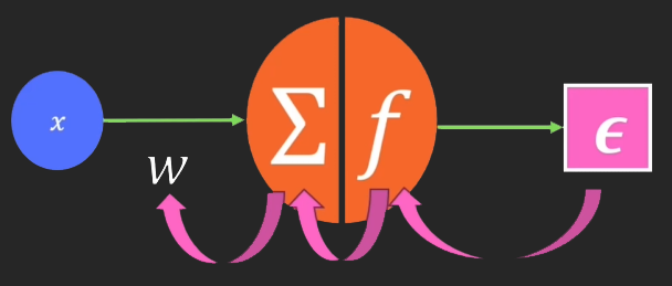

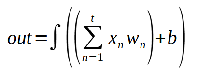
Are you sure we need to do this? Doesn't what we've already implemented perform the task shown in the previous image? No, dear reader. In fact, what we've implemented so far doesn't allow us to use an activation function. This is precisely the step we still need to implement. Essentially, up to this point, we have implemented only the most basic part of the loss function for adjusting the weights and bias. Thus, the calculation that we have been performing so far for both the least squares method and the gradient method is shown in the following figure.

As you can see, this expression contains a constant equal to one. It is precisely this constant that constitutes the activation function. Since the activation function is not used during backpropagation, the derivative that would otherwise need to be computed for this function becomes a constant, which in this case is equal to one. However, when activation functions are added, this constant changes. This gives us the expression shown below.

This raises an interesting question that many people find difficult to understand, perhaps because there is no truly adequate explanation of this topic. It might seem obvious what's going on inside. However, unlike backpropagation—in which the expression given above is used during the training of a perceptron—the most important function is not the one represented in that expression, but the one we will see below.

This is the expression we actually use—both when we already have a trained model and during training. Just to clarify: the integral symbol you see in this expression does not mean that we will be evaluating the integral. It is used solely to represent the activation function. If you take a closer look at this expression, it becomes clear that it does not involve any complex calculations. It all comes down to addition and multiplication—and, of course, one of the activation functions described in the previous article. This function must be defined when creating the perceptron so that everything works correctly.

And now for the most interesting part. You're probably already thinking, "So does that mean a perceptron has two outputs instead of one? Is this what we just created?" Yes, that's exactly what will happen. However, we haven't created those two outputs yet. Indeed, backpropagation can already be regarded as one of the outputs, but in its current form, it does not yet count as one. One is known as forward propagation, and the other as backpropagation. Both must be present for the perceptron to be truly useful to us.

Since this concept is very simple and seemingly obvious, forward propagation is rarely discussed. By contrast, backpropagation is discussed extensively, even if the explanation remains somewhat incomplete.

Concluding Thoughts

In this article, I explained in more detail how and why the gradient came to be used in perceptron networks. We have also begun to explore another topic: forward propagation and backpropagation, although we haven't yet added activation functions to the perceptron to see this mechanism in action. What we have covered here will make the material in subsequent articles easier to present and, consequently, easier to understand.

Although all of this may seem a bit far off for now, we're moving in the right direction. Therefore, I ask that you carefully study this material, as understanding what is presented here is essential to understanding what we will discuss next.

MQ5 File	Description
Scripts\Example A	Basic Demonstration
Scripts\Example B	Basic Demonstration