Neural Networks in Practice: Activation Functions

I know that many people may think it’s unnecessary to understand the activation function graph and its derivative, and that we could dive right into the topic, leaving such questions aside. However, it's much easier to understand why the sigmoid function can't be used in very deep networks if you understand its graph.

Everything stated in the previous article still holds true. In addition to what we saw there, we'll take a look at some new code here. We'll also briefly explain each of the selected functions. Before I begin, I'd like to remind you of something, dear reader. There are a vast number of activation functions. Some of them are more popular than others. Nevertheless, each of them has its own purpose and specific area of application, helping to optimize training speed in one way or another. Next, we'll look at how some of these functions are used in practice, so you can see just how much even a simple change in the choice of function can affect the results we obtain during network training. In any case, for now we'll focus only on the truly interesting part of the system, where we'll use the functions in complete isolation. That will make it easier to understand which option might be best in different situations. In any case, don't worry about it right now. Although the mathematical part is quite complex and confusing, we'll try to simplify it considerably by the end. I want you to really understand how a neural network works. The point isn't to tell you, "Do this. Don't do that." Instructions like these don't add anything to your knowledge. This merely creates an illusion that you understand something you actually don't.

Yes, this code does look significantly more complex. But don't worry. I'll explain each part so you can understand it. It's actually simpler than the previous code. First, an enumeration was added on line 8. Its purpose is to allow us to select the appropriate equation. Each of the names included in this enumeration actually corresponds to the name of an equation.

These six equations are used in activation functions. As I mentioned earlier, there are others as well. Many of them are slight variations of the ones listed here. If you'd like, you can add them without any problem. You only need to take one precaution: put the mathematical expression in the right place and in the correct form. If you do this, you'll be able to plot a graph for any mathematical function you want. And it's all quite simple and straightforward.

So, now that we have names for the equations, the next change concerns how the user selects an equation to plot. In the past, we had to compile the code every time we made changes—whether to the equation or to the parameters used. However, as I mentioned at the beginning, the goal here is to provide the user with a more interactive experience. This way, you won't have to constantly compile the code. Four input parameters were provided for this purpose. Previously, we had two: the range of values and the plotting step. Now two more have been added: equation selection and the Y-axis scale factor. This is because, in some cases, the values on the Y-axis are very close to 1.0. In that case, it would be a good idea to let the user change the scale of the Y-axis. This will change the scale of the graph, making it easier to analyze the plotted curve.

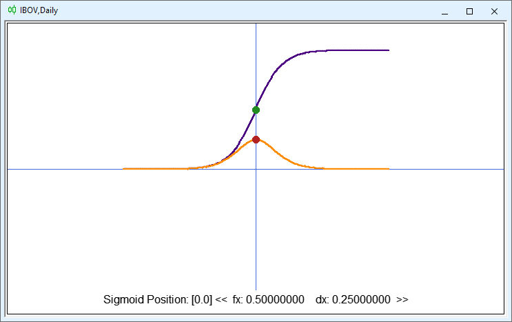
Please note that some changes have been made to the display. In fact, the change affected only the part related to the displayed text. Previously, we only displayed the position along the X-axis. Now, in addition to this value, we also display the name of the equation, its value on the Y-axis as a function of the value on the X-axis, and the value of the derivative at that same point on the X-axis. And all of this was achieved by changing just a few lines of code. Essentially, line 39 of the code displays the fx and dx values you see in the image. Please note that in this line, we access the enumeration to retrieve the function name. We also access the values specified in line 31. These two variables in line 31 did not exist before.

So, since most of the code remained unchanged, the only changes were the addition of lines 151, 152, 185, and 186, which are intended to make the chart window as clean as possible. Since this is easy to understand, we can focus on what's important: the procedure on line 44.

If you compare this code to what we looked at in the previous article, you'll immediately notice that two new variables have been added here. They are on line 48. Even the variables fx and dx now serve a different purpose. Now both variables will be used to temporarily store the calculated values.

This may seem complicated, but if you've never programmed before, pay close attention—because you're about to learn how to do it in just a few steps.

Let's say you want to add a new activation function to this application so that you can graph both the values calculated by its equation and its derivative. What should you do? So, to start, go to line 8, where the function names are listed, and add the name of your new function. Remember that you CANNOT use spaces in the name. If you need to separate words, use the underscore ( _ ).

After that, you will be able to select this equation when using the compiled application in MetaTrader 5. However, you won't see any graph just yet. To plot the function, simply go to the procedure shown in the previous code snippet and do the following: locate the switch statement on line 60. It will determine which code to execute based on the value corresponding to the equation selected by the user.

So, on line 61, after the opening curly brace, press ENTER, type "case" followed by a space, and then type the name of your equation followed by a colon ( : ). Press ENTER again and type "break" followed by a semicolon ( ; ). This will create a structure very similar to the one shown in the code. And now for the most interesting part. Between the colon ( : ) and the word “break,” you need to write something very similar to what is shown in each of the structures between lines 62 and 86. Note that fx is assigned one value and dx another. So what does that mean? For fx, you need to specify the expression for the function, and for dx, the expression for its derivative. And that's all you need to do. The rest is handled by the code itself or during its use in MetaTrader 5. If you're not sure how to use the switch statement, check out another article I wrote. In that article, I explain in detail how to use the switch statement.

This function has already been discussed in another article, where I showed that an activation function is needed to overcome stagnation. Check out the previous articles to gain a better understanding of this topic. So, when we add the indicator to the chart and select the sigmoid function, we'll be able to interact with the chart as shown in the following animation.

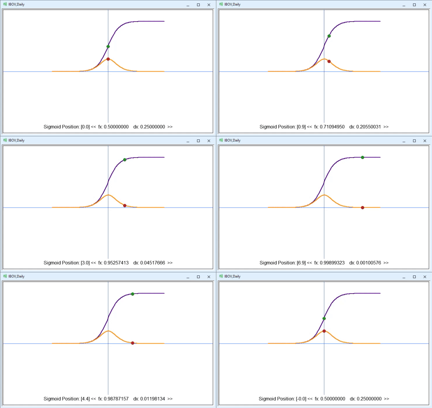
However, if you simply look at these mathematical expressions, you might not immediately notice just how much the derivative of the sigmoid function reduces the values. To some extent, this is rather inconvenient, as it has significant implications when we want to use this function in a deeper network. We need to be careful when deciding at which point in the network we will use the sigmoid function. If you use it indiscriminately, at some point you'll prevent the network from continuing to propagate data. This will become clearer later. Anyone with even a basic understanding of math and derivatives is probably already thinking about the next topic: THE CHAIN RULE. That's what this problem is called. However, this actually affects us only when using derivatives and only during backpropagation. As I mentioned earlier, we'll go over all of this in more detail later.

Even with this issue in mind, the sigmoid function is extremely useful because it normalizes the perceptron's output values, keeping them within the range of zero to one. In addition, it is often used when we need a model that can predict the probability of something based on a neural network's output value. Since the output value always falls within the range from zero to one, it is ideal for converting data into percentages. The sigmoid function has another major advantage, provided it is used with caution: it helps avoid abrupt changes during gradient descent. This is because this function is differentiable, which means we can determine the slope of the curve using any two points.

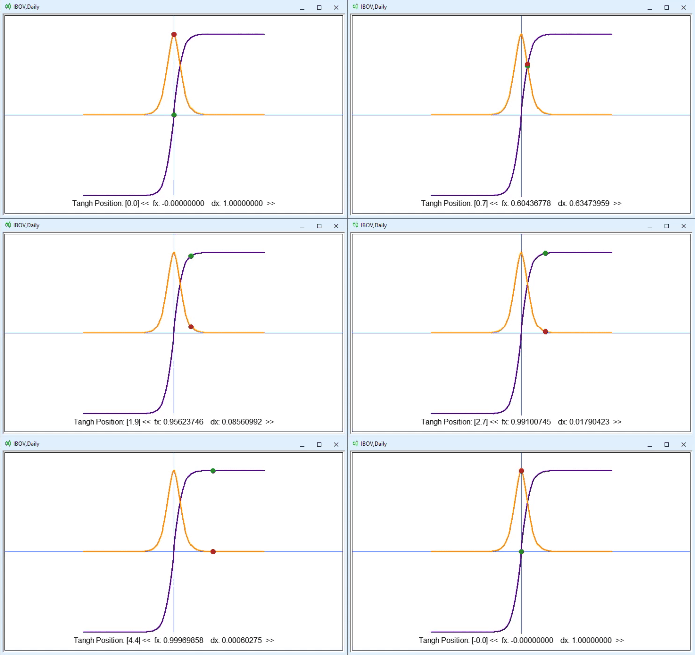
This activation function attempts to address one of the problems with the sigmoid function: its output cannot be negative. Furthermore, in some cases, the fact that the sigmoid function is restricted to values between zero and one creates an additional complication. This is noticeable when its values approach zero. In many cases, this effect can be devastating for a perceptron network, as it essentially “kills off” some of the weights being used, causing them to be completely ignored, even though they could actually help classify new data entering the network.

So, when you select the “hyperbolic tangent” function in the app, you’ll see the following animation.

As for the equation, there are slight variations in its notation. One of these appears on line 67 of the code and is shown below.

There is another way to write this same equation. You can see it below.

In the previous equation, you can clearly see that, contrary to what many people think, trigonometric expressions can be used in perceptron networks. Sometimes using trigonometric equations offers far more advantages than you might imagine, since they can be derived using well-known trigonometric identities. However, the previous example was just an interesting aside. Below is another way to write the same expression.

Despite these differences in how the equation is written, the part relating to its derivative does not change significantly. Nevertheless, there are several ways to express it. In the code, you can see the derivative on line 68, where the equation shown below is used.

We can also use an equation similar to the one shown below, which also allows us to find the derivative.

Of course, these expressions represent only a small selection of the many different ways to express the same thing. In other words, you shouldn't blindly follow formulas or expressions you find somewhere just because someone said they're the best option. As I mentioned earlier, humanity does not yet know exactly how to build a universal perceptron network. The only thing we've managed to figure out is how to create a network that adapts more or less adequately to a specific type of task.

All right, let's continue, because there's still more to show in this article.

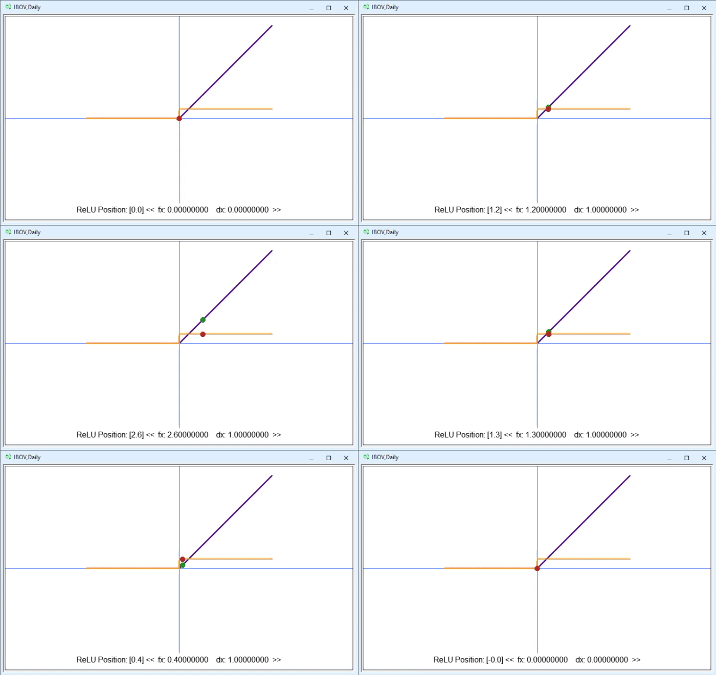
We already discussed this function in the previous article. So we'll quickly go over it here. When you select it, the following graph will appear, and we'll be able to interact with it.

This is one of the many existing variations of the ReLU function. It was mentioned in the previous section specifically so that we could show its mathematical expression here. If you have never encountered variations of mathematical expressions, this will let you compare one such variation with the original expression, so to speak.

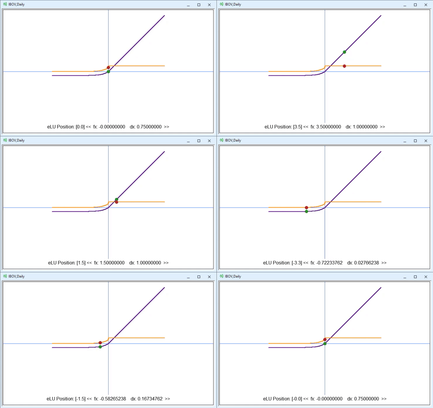
"Oh my God, we're definitely going to have to call an exorcist for these two expressions. How terrifying." Well, regardless of what you're thinking right now and how much these expressions might scare you, there's something they both have in common: the Greek letter ALPHA. It is located on line 75 of the code. The purpose of the alpha parameter is to adjust the curvature of the graph. Depending on the value you set, you can get a steeper or a gentler curve. In other words, the radius of the arc you see on the graph may be slightly smaller or larger. This results in a slight difference in the perceptron's output values. However, if we look at both expressions, we can see that, unlike the original ReLU function, the eLU function does not have any issues with zero, since the equation itself can handle a zero value in the derivative.

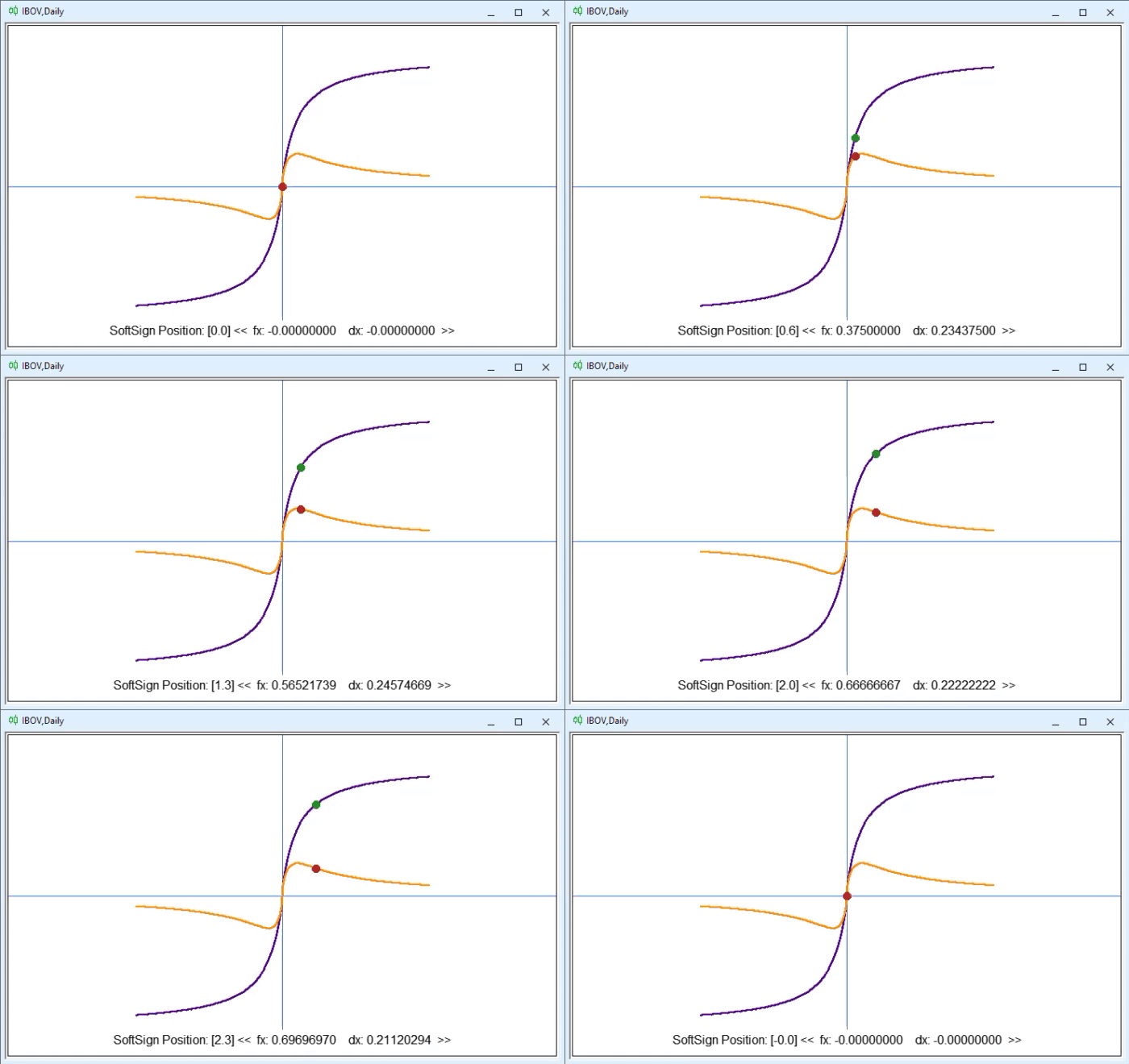
If you look closely, you'll notice that SoftSign lies somewhere between the sigmoid function and the hyperbolic tangent. However, in certain situations, it may prove to be much more suitable than either of them. Depending on the problem you want to solve, it can help the gradient find the minimum somewhat more efficiently than the sigmoid function or the hyperbolic tangent. In addition, because of how it is calculated, this function can be faster to compute in deeper networks. In some cases, this makes a noticeable difference during training. Models that use TensorFlow often favor this function over the sigmoid function and the hyperbolic tangent precisely because of this factor during model training.

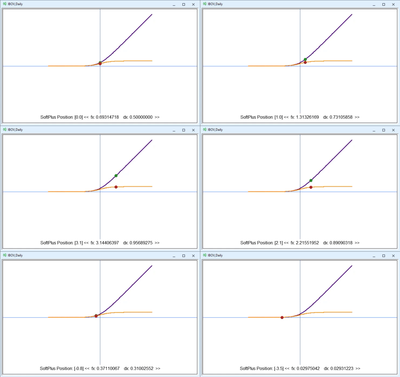
You can clearly see that it smooths out the transition between negative and positive values quite significantly, following the same principle as the original ReLU. However, unlike the original ReLU and eLU, which we just discussed, SoftPlus behaves much more gently and smoothly. In other words, starting at a certain value, the transition near zero becomes much smoother. This differs from ReLU, which simply switches abruptly to zero or one depending on whether the values are negative or positive.

I have to admit, the final result in this article surprised me, as it turned out to be much more interactive. You don't need to make major changes to the code to add new functions for exploring possible mathematical models. All you need to do is add the name of the equation, followed by its mathematical expression.

Thus, in this article, you have not only seen how different activation functions affect the perceptron's output in different ways, but you have also learned that even small changes in the way calculations are performed can significantly influence the choice of activation function. Keep in mind that not all perceptron networks use functions like the ones shown here. However, we'll talk about that another time.