Neural Networks in Practice: ReLU Function Graph

Introduction

In the previous article, “Neural Networks in Practice: The Birth of C_Neuron”, we began to take a slightly more organized approach. We began creating a class designed to contain everything we'll need to include in the neuron. In the future, this will allow us to connect several neurons into an architecture intended essentially to form a small, simple neural network. Nothing on the level of ChatGPT or anything like that. The goal here is to show neural network enthusiasts how neural networks work internally. Without using any additional resources. By programming everything ourselves.

So, our first basic neuron is already capable of doing certain things, since it converges in many simple test scenarios. The fact that it already lets us change the number of inputs extremely easily and quickly makes it much more interesting in terms of its potential applications. However, it is still in the very early stages. Its model does not yet include activation functions or a structure that would allow us to connect neurons in series, thereby forming a sequence of neurons and, consequently, a small neural network.

But before we get into that, we need to talk about something else. So, here we'll start by talking a little bit about activation functions. In many cases, most beginners in neural networks use these functions incorrectly. The reason for this misuse is that these functions are misunderstood and, in many cases, poorly explained overall.

Some people simply say that you should use one activation function or another, and that in itself is a mistake. But the worst part is that users of these functions don't even have a basic understanding of the math involved. And when such a person sees that their neural network has stopped learning, they can't figure out why. As a result, they make the wrong decisions precisely because they lack knowledge of the relevant mathematics.

What happens inside the activation function is exactly what I will explain in this article, although this will most likely require further articles as well. The idea is for you, dear reader, to understand when, why, and how to use and choose the most appropriate activation function. Every case is unique. There is no one-size-fits-all solution or anything that you should always do or use. However, to make the best decisions, it is necessary to understand how each activation function works and how it affects the entire neural network.

Well, since there are literally dozens of activation functions, I'll show you just a few of them. At least the most popular ones—or the ones used in most cases. So don't assume that the only functions that exist are the ones that will be shown and explained here. Look for information about mathematical expressions or equations that can be used as activation functions. But, at the very least, I'll try to give you a foundation for understanding the basics of this topic—one that many people talk about but few truly understand.

Understanding the Problem

When trying to explain certain things, a problem arises. It's not because they're difficult. That's not the case at all. Often, the problem is that we need to understand several elements that seem unrelated but are actually part of a single whole. The topic of activation functions—as well as backpropagation, which I'll discuss later—is one such case. It is very difficult to explain how this works without touching on certain issues that may not yet have been properly addressed.

So, to put it very briefly, the activation function serves to clip and modify the secant line generated by the loss function. That's basically it. It may seem crazy to put it this way, but the activation function has no other purpose than the one I just mentioned. And no, the loss function uses a secant line, not a tangent line. I've already explained this in other articles. But that's only the simple part of the explanation. The challenge lies in showing how the activation function produces this effect and why, in some cases, we really do need it, while in others we can easily do without it. This contradicts the fairly common assertion that a neural network must always use some kind of activation function.

Well, I think it makes perfect sense to focus the explanation on showing how all of this works. However, there is another problem that arises because we are using gradient descent instead of the least squares method. We will discuss this issue in greater detail when we move on to backpropagation, but even now it requires a certain degree of caution when choosing an activation function. So what exactly is the problem? Well, the problem stems from derivatives.

But how is that possible? Don't derivatives serve to reduce the computational cost of the loss function? Yes, dear reader. However, when we use derivatives in the loss function, we need to consider how they will affect the activation function. As I just mentioned, this problem is particularly evident during backpropagation. It is precisely here that the use of derivatives takes on special significance. This is because if you choose the wrong activation function, at some point the neuron—or, more precisely, the neural network—will simply stall. Due to a mathematical error, the network will no longer be able to converge. In other words, you might think you know what you're doing, while your neural network simply stops working precisely because of a lack of mathematical knowledge in this area.

Consequently, what I am about to explain here applies only if we use derivatives in the loss function. If you aren't using derivatives, most of what will be explained will not apply to your neural network. Now that we've cleared that up, we can start breaking everything down in a way that's as clear and easy to visualize as possible. The main point is that the explanation will involve quite a bit of math. So anyone who doesn't like math is sure to hate this topic. But, unfortunately, that's exactly how neural networks work. There's a lot of math here, and just when it seems like it's all coming to an end, it starts all over again—only with even more math.

It is practically impossible to explain anything using very little math. Nevertheless, we'll start with a very simple activation function whose underlying math is also very simple. That way, dear reader, you won't be intimidated by what we'll cover next.

Rectifier Activation Function

So, the first activation function we'll look at is the Rectifier, better known as ReLU. But where did the name "ReLU" come from? It comes from its full name: REctified Linear Unit. It is precisely these capital letters that are used to form the name. That's where the name ReLU comes from. Its goal is very simple: to eliminate all negative values in the neural network. That's exactly right. In certain cases, negative values can do us more harm than good. In other cases, however, they are necessary to ensure proper convergence of the neural network's parameters. If your particular network has problems with negative values, you can use ReLU to eliminate those values. Its formula is given below.

But tell me, is that really all the activation function does? Yes, dear reader. However, a problem arises when we use derivatives in the loss function. Just to clarify: whenever I talk about derivatives, I mean derivatives of the loss function, unless I explicitly state otherwise. That way, I'll avoid constantly repeating the same term.

But let's get back to the topic. If you're familiar with the basics of derivatives, you know that the derivative cannot be defined at zero. And this is one of the problems that arise when using ReLU. Any negative value is automatically converted to zero. And when we have to calculate the derivative at that point, a problem will arise. Again, the problem doesn't arise now, but during backpropagation.

However, the derivative of this function is very simple. In fact, it is one of the simplest derivatives of any activation function. The equation is given below.

The expression above gives the result of calculating the derivative. But note the following: we define a value for x less than zero and for x greater than zero. What happens when x equals zero? Well, in that case, the value will be undefined. But in computing, you can't work that way. That's why we have to resort to a little trick or workaround. When x is equal to zero, we determine the value of the derivative ourselves. It is usually defined as zero. But that doesn't mean it's actually equal to zero. It's just a workaround used in calculations. So, that was the mathematical part of the explanation. But as programmers, we aren't all that interested in this mathematical notation. To tell the truth, some of this notation looks like hieroglyphs—they're so confusing and difficult to make sense of. I apologize to any mathematicians here, but I couldn't resist making that joke.

All right, now, to make this a little more visual, we'll implement a small indicator that lets us explore these functions more easily by viewing them on a chart. That way, I think it will be much easier to understand what's going on. We could use different languages to plot function graphs, but since the goal is to do everything in MQL5, we'll do it entirely in MQL5. That'll be interesting. However, to keep the topics somewhat separate, we'll cover this in a new section.

Graphical Representation of Functions

Since many people find it very difficult to look at an equation or a mathematical expression and understand it, I believe that presenting it graphically is much more intuitive and helpful for learning. This way, you can study both the function graph and the code used to create it. The code we'll look at is designed to make it easier to understand what this mathematical equation represents.

So, with that in mind, let's take a look at the source code for our indicator. It is provided below.

001. //+------------------------------------------------------------------+
002. #property copyright "Daniel Jose"
003. #property indicator_chart_window
004. #property indicator_plots 0
005. //+------------------------------------------------------------------+
006. #include <Canvas\Canvas.mqh>
007. //+------------------------------------------------------------------+
008. #define def_Limit   10.0
009. #define def_Step    0.5
010. //+------------------------------------------------------------------+
011. CCanvas *canvas;
012. //+------------------------------------------------------------------+
013. struct st_00
014. {
015.     int     x,
016.             y,
017.             maxX,
018.             maxY;
019.     double  Position;
020. }global;
021. //+------------------------------------------------------------------+
022. void PlotTextPosition(void)
023. {
024.     uint w, h;
025.     string sz0;
026. 
027.     sz0 = StringFormat("Position: [%.1f]", global.Position);
028.     TextGetSize(sz0, w, h);
029.     (*canvas).TextOut(global.x - (w / 2), global.maxY + 5, sz0, ColorToARGB(clrBlack)); 
030. }
031. //+------------------------------------------------------------------+
032. void Function_Curve(void)
033. {
034. }
035. //+------------------------------------------------------------------+
036. void UpdateGraphics(int direct)
037. {
038.     double value = global.Position + def_Step * direct;
039. 
040.     global.Position = MathAbs(value) <= def_Limit ? value : global.Position;
041. 
042.     (*canvas).Erase(ColorToARGB(clrWhite, 255));
043. 
044.     (*canvas).LineVertical(global.x, 0, global.maxY, ColorToARGB(clrRoyalBlue, 255));
045.     (*canvas).LineHorizontal(0, global.maxX, global.y, ColorToARGB(clrRoyalBlue, 255));
046. 
047.     PlotTextPosition();
048.     Function_Curve();
049. 
050.     (*canvas).Update(true);
051. }
052. //+------------------------------------------------------------------+
053. void Resize(void)
054. {
055.     uint w, h;
056.    
057.     global.maxX = (int)ChartGetInteger(0, CHART_WIDTH_IN_PIXELS, 0);
058.     global.maxY = (int)ChartGetInteger(0, CHART_HEIGHT_IN_PIXELS, 0);
059. 
060.     if (canvas != NULL)
061.     {
062.         (*canvas).Destroy();
063.         delete canvas;
064.     }
065.     canvas = new CCanvas;
066.     (*canvas).CreateBitmapLabel("BL", 0, 0, global.maxX, global.maxY, COLOR_FORMAT_ARGB_NORMALIZE);
067.     global.x = global.maxX / 2;
068.     global.y = global.maxY / 2;
069.     TextGetSize("M", w, h);
070.     global.maxY -= (int)(h * 2);
071. }
072. //+------------------------------------------------------------------+
073. int OnInit()
074. {      
075.     ZeroMemory(global);
076.     canvas = NULL;
077. 
078.     return INIT_SUCCEEDED;
079. }
080. //+------------------------------------------------------------------+
081. int OnCalculate(const int rates_total, const int prev_calculated, const int begin, const double &price[])
082. {
083.    return rates_total;
084. }
085. //+------------------------------------------------------------------+
086. void OnChartEvent(const int id, const long &lparam, const double &dparam, const string &sparam)
087. {
088.     int direct = 0;
089. 
090.     switch (id)
091.     {
092.         case CHARTEVENT_CHART_CHANGE:
093.             Resize();
094.             break;
095.         case CHARTEVENT_KEYDOWN:
096.             if (TerminalInfoInteger(TERMINAL_KEYSTATE_LEFT)) direct = -1;
097.             if (TerminalInfoInteger(TERMINAL_KEYSTATE_RIGHT)) direct = 1;
098.             break;
099.     }
100.     UpdateGraphics(direct);
101. }
102. //+------------------------------------------------------------------+
103. void OnDeinit(const int reason)
104. {
105.     (*canvas).Destroy();
106.     delete canvas;
107. }
108. //+------------------------------------------------------------------+

This code provides the basic foundation for what we'll need and what we'll be using. Right now, it does almost nothing. It simply creates a representation of the Cartesian plane on the chart and displays a short message. In addition, of course, it allows us to interact with the chart to some extent. In other words, something truly simple and basic. However, for those who look at this code and can't figure out how it works, we'll briefly break down its key points. This way, you, dear reader—who may have come to this article simply as an enthusiast without much background—will find it easier to understand what we're doing in this very simple code.

Basically, there are two places in this entire code that you can change if you want to. There's one more place, but we'll get to that later. Basically, you won't need to change anything.

But if you decide to make a change, I recommend focusing on the following points: first, the value specified in line eight, and second, the value specified in line nine. These values are used to set the offset of the indicator, which will subsequently be placed on the chart. Essentially, these are the only two parameters you can change at this point.

So, let's take a quick look at this code to understand its other details. In line 11, I declare a variable that will be used to access the MQL5 Standard Library. Please note that I am declaring this variable as a pointer. And there's a reason for that. By defining it this way, I'll be able to check whether the object has been initialized.

On line 13, we define a global structure whose purpose is to provide more controlled access to certain variables. On line 22, we have a procedure that allows us to display certain information as text. In this case, we will display only the value of the current position. Line 32 contains a procedure that we'll discuss later. However, that will depend on exactly what we place on the chart. Line 36 contains a procedure designed to update the chart whenever changes are made to it. It's very simple and doesn't require any special explanation.

Now, on line 53, we see a rather interesting procedure. Essentially, this procedure adjusts the dimensions of the bitmap object we are using through the MQL5 Standard Library. The entire procedure is quite simple. However, on line 60, we check whether a CCanvas class instance has been created. If an instance has already been created, we'll remove it from the chart, and then, on line 65, we'll initialize the pointer to create a new instance of the class. That is exactly why I use a pointer in the declaration on line 11. But why am I doing all this? To understand this, you need to understand how MetaTrader 5 actually executes an indicator.

When we tell MetaTrader 5 that we want to add an indicator to the chart, MetaTrader 5 begins executing the code starting with the OnInit function, located on line 73. In this function, we initialize various elements. For example, on line 75, we initialize the global variables, ensuring that they all start at zero. And on line 76, we set the pointer to null. In other words, it doesn't point to any instance. After that, MetaTrader 5 generates a new event, which will be handled by the function on line 86. The first event is CHARTEVENT_CHART_CHANGE, which notifies all applications on the chart that something has changed. Since our application handles this event, on line 93 we will call the procedure defined on line 53. This is precisely when we begin creating a CCanvas class instance from the MQL5 Standard Library: the instance is created on line 65.

Okay, but was all that complexity really necessary? In fact, this does not add complexity. If you resize the chart, MetaTrader 5 will generate the CHARTEVENT_CHART_CHANGE event again. This allows us to always maintain the correct dimensions without having to constantly check each item. But, getting back to the explanation, on line 81 we have the OnCalculate event handler. It won't do anything, but it needs to be declared because our application is an indicator. The OnChartEvent event handler is located on line 86. As we've already seen, it is used during initialization or when changes occur on the chart. But it also allows you to process presses of the right and left arrow keys, thereby changing the position, as we'll see shortly.

Line 103 contains the procedure responsible for handling the Deinit event, which will remove all elements placed by the application that are not intended to remain on the chart. If you compile this code and run it on any chart, you'll see the following animation when you press the right and left arrow keys.

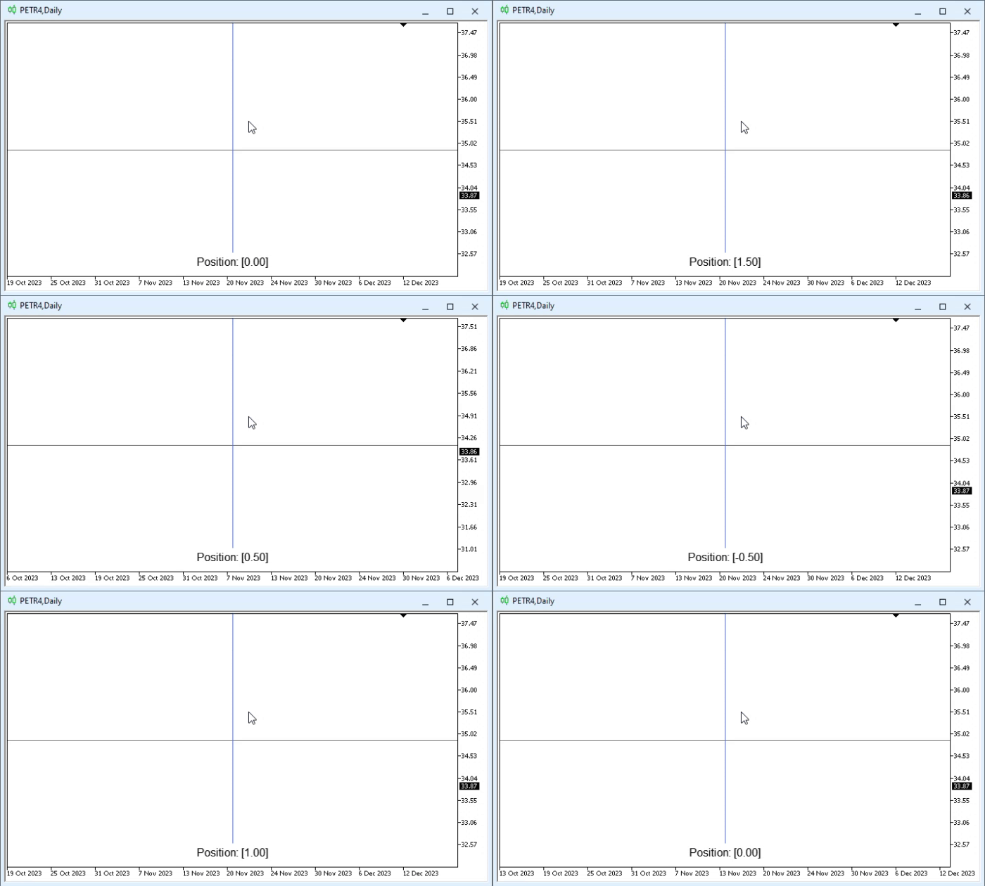
This is a very interesting idea because now all we have to do is specify the expression or equation we want to plot on the chart. After that, we'll be able to visualize it with virtually no changes to the code. However, this raises an interesting question. We need to describe this equation using code, rather than in mathematical form. However, if we developed a system specifically designed for this purpose, we could write the formula exactly as it is usually presented in textbooks and mathematical literature. Since our goal here is simply to highlight a few details, we won’t go that far. We'll stick to the basics.

So, now we need to think about how we're going to display the curves on the chart. In other words, we need to add some code to the procedure on line 32. This is probably the most interesting part, since there are different ways to do it. But since I want to use as little code as possible, we'll do this using a technique I used when I was just starting out as a programmer. It's a relatively simple mechanism, but it allows us to accomplish a lot with minimal effort, even on less powerful computers.

So, let's see how the curves will be displayed; at first, they won't be very smooth. However, you'll see that we can go much further; it all depends on what we want to achieve. Remember that to make the curves smoother, all you need to do is change the values in lines 8 and 9. You'll understand this point better soon. So, let's take a look at the code. And since only this section will differ for each of the activation functions shown, I will divide it into blocks or sections. So, let's take a look at the first of these functions in the next section.

Displaying ReLU and Its Derivative

The code below shows how to display both the ReLU activation function and its derivative.

31. //+------------------------------------------------------------------+
32. void Function_Curve(void)
33. {
34.     int x[], y[], d[];
35.     uint p;
36.     double fx, step;
37.     
38.     ArrayResize(x, (int)(((def_Limit * 2) / def_Step) + 1));
39.     ArrayResize(y, x.Size());
40.     ArrayResize(d, x.Size());
41. 
42.     step = MathMin(global.maxY, global.maxX) / (x.Size() * 1.0) / def_Step;
43. 
44.     fx = -def_Limit;
45.     for (uint c = 0, m = x.Size(); c < m; c++, fx += def_Step)
46.     {
47.         p = (fx <= global.Position ? c : p);
48.         x[c] = global.x + (int)(step * fx);
49.         y[c] = global.y - (int)(step * MathMax(0, fx));
50.         d[c] = global.y - (int)(step * (fx <= 0 ? 0 : 1));
51.     }
52. 
53.     (*canvas).PolylineThick(x, y, ColorToARGB(clrIndigo, 255), 3, STYLE_SOLID, LINE_END_ROUND);
54.     (*canvas).PolylineThick(x, d, ColorToARGB(clrDarkOrange, 255), 3, STYLE_SOLID, LINE_END_ROUND);
55. 
56.     (*canvas).FillCircle(x[p], y[p], 5, ColorToARGB(clrForestGreen, 255));
57.     (*canvas).FillCircle(x[p], d[p], 5, ColorToARGB(clrFireBrick, 255));
58. 
59.     ArrayFree(d);
60.     ArrayFree(y);
61.     ArrayFree(x);
62. }
63. //+------------------------------------------------------------------+

Great, here's some excellent code. It even seems almost divine, because you can really accomplish a great deal with just a small amount of code. And all of this is done in an extremely simple and clear way. But, first and foremost, it's easy to explain, which makes it quite intuitive, even though it isn't particularly efficient in terms of performance. Let's take a closer look at what's going on here. But first, let's look at the result of running the code. You can see this in the following animation.

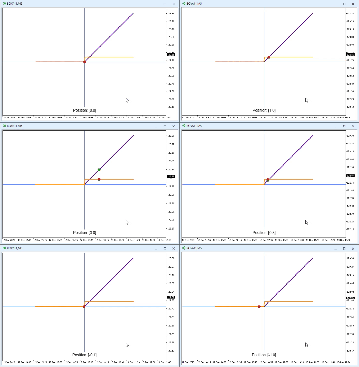
It's truly impressive what we can accomplish when we're really ready to take it on. Okay, but let's take a closer look at what this animation shows. To do this, we should take another look at the excerpt shown at the beginning of this section. So, let's take a closer look at the details. In the animation, you can see two line segments: one is indigo—a shade of blue—and the other is orange. You can also see two round shapes: one is green, and the other is red. These objects are created by the following lines, respectively: 53—the indigo line, 54—the orange line, 56—the green circle, and finally, 57—the red circle.

Please note that all of these lines have something in common. All of them use, in one way or another, the arrays declared on line 34. So, let's take a look at how the various elements are drawn on the screen. This is important because most of the code shown in this snippet will remain unchanged. We'll only need to change two lines to display the remaining activation functions.

So, in lines 38–40, we allocate enough space to store all the values within the range specified in line 8. In line 42, we calculate the step size—or, in other words, the resolution—at which the curves will be plotted. Since this value depends on both the size of the graphics window and the values specified in lines 8 and 9 of the code, we may need to adjust some parameters slightly to get a curve that displays properly. If the plot is too coarse, you'll notice that the curve appears very jagged when it's rendered. Since ReLU is essentially a straight line, we can't see this problem yet, but you'll clearly see it a little later.

Since this part of the code won't change, you'll only need to change the value on the ninth line to increase the resolution and make the curve display more smoothly. In any case, on line 44, we initialize the value of fx. This is the value that will be used in the calculations. Next, we move on to the for loop on line 45. This loop does practically all the work, since it is responsible for creating curves or lines, depending on the specific case.

On line 47, we perform a simple search to determine the index in the array. This index will be used to display the circles on the chart. But why is it done this way? The reason is quite simple: to avoid unnecessary repetition of calculations. Without line 47, we would have to perform the calculations twice: once to plot the graphs of the function and its derivative, and a second time to determine where to place the points on the curve so we can see where sampling takes place. Line 48 contains the calculation that determines where the points will be located on the X-axis. These points depend on both the limit and the number of divisions. Both values are declared in lines 8 and 9 of the code.

Great, now let's take a look at the only two lines we'll need to change to plot different functions. I would like you, dear reader, to pay special attention to lines 49 and 50. Notice that they are practically identical except for their endings. Do you know what that means? So, if you've read the article carefully, you'll notice that the end of line 49 matches exactly the calculation for ReLU shown above. In turn, the end of line 50 contains the calculation of the derivative of the ReLU function. It may seem surprising that these calculations are so easy to express in code, but it's true. So much so that absolutely all of the code will remain unchanged, regardless of the situation. The only thing that will change is the content of lines 49 and 50.

That's great—it turned out perfectly. Finally, we use line 53 to plot the curve of the calculated function, and line 54 to plot the curve of its derivative. In line 56, we place a small circle on the curve of the function, and in line 57, we place another circle on the curve of the derivative. That really is amazing. Without resorting to any particularly clever code tricks, we managed to create something capable of plotting the function graphs of a function and its derivative so that we can interactively analyze what happens at each point on the curve. That's just wonderful.

Concluding Thoughts

In this article, we essentially limited ourselves to writing the code entirely in MQL5 so that we could take our time exploring derivatives and the corresponding functions. Understanding what happens to the value of the derivative or to the function itself will be extremely important for understanding how activation functions actually work. But first and foremost—to understand when and why to use a particular activation function.

Since a significant portion of this article was devoted to demonstrating the indicator we will use to visualize the derivative curve and the activation function curve, only the ReLU activation function is available in the attached file. However, we'll soon take a look at other activation functions as well. If you, dear reader, already know which equation to use, you can implement it directly in your code. But if that's not the case, don't worry. We'll go through, one by one, at least the most popular—or most frequently used—activation functions. This way, you can take your time exploring each one, experimenting and observing how it changes as the values change.

In any case, make use of the information provided in this article. And for homework, why not create a grid on the Cartesian plane? It's not hard to do. Nevertheless, I'll leave this as an exercise so that everyone can try to implement it as best as possible. The idea is to be able to see the values along the X and Y axes by moving the small circles along the curves.