Neural Network in Practice: Sketching a Neuron

Introduction

Hello everyone and welcome to another article about neural networks.

In the previous article Neural Network in Practice: Pseudoinverse (II), I discussed the importance of dedicated computational systems and the reasons behind their development. In this new article related to neural networks, we will delve deeper into the subject. Creating material for this stage is no simple task. Despite appearing straightforward, explaining something that often causes significant confusion can be quite challenging.

What will we cover at this stage? In this series, I aim to demonstrate how a neural network learns. So far, we have explored how a neural network establishes correlations between different data points. However, the methods discussed until now are only applicable when working with a pre-processed and filtered dataset. This allows the neural network to identify optimal solutions based on existing information. But what happens when the data is unfiltered? How does a neural network establish correlations in such cases? This is where many people mistakenly believe that a neural network possesses some form of intelligence. They assume it "learns" how to classify things in an autonomous, human-like manner.

This common misconception makes explaining neural networks particularly challenging. Often, those who seek to understand them lack the basic knowledge of how to sort through different types of information, even if the data has some relationship to each other. This is the most confusing point for those who do not work with it. As a result, they may misinterpret explanations, leading to further confusion about how neural networks function.

To clarify, I am not suggesting that neural networks learn in the way humans do. There is no hidden intelligence within them. Anyone who believes otherwise is mistaken. A neural network is nothing more than a complex mathematical equation. However, this equation has the remarkable ability to analyze and classify data. Once a dataset is classified, any new data point similar to an existing classification will be assigned a probability of belonging to a known category.

This concept has been covered in previous articles, but here, we will take a slightly different approach. This approach is something that is both fundamental and intriguing. We will start from the absolute basics and progressively build up to constructing a neural network using artificial neurons.

The Fundamentals

To really understand how a neural network learns when we show it information, I ask you to forget everything you think you know about artificial intelligence and neural networks. Much of what you (think) you know is likely pure nonsense or misinformation, especially if you've seen it on news sites or other such sources. The topic of neural networks came into the public eye mainly because some entrepreneurs saw them as a money-making opportunity, but neural networks have been in development for decades. They are neither new nor function in the way they are often portrayed. While highly useful, they are primarily relevant to those with a strong interest in programming.

At their core, all neural networks (which some refer to as artificial intelligence) are based on a simple mathematical principle discussed in previous articles. Here we will look at this concept in more detail. This is the secant line. Regardless of what others claim, everything in neural networks boils down to this fundamental concept - finding a secant line that approximates the tangent line. It's actually quite simple.

In previous discussions, we bypassed this step and jumped directly to identifying the tangent line. This explains the formulas introduced earlier. Those formulas were specifically designed to shortcut the process and arrive directly at the tangent line. All this material relates to a very specific fact: when we have filtered, selected information in our database. When this happens, we don't need a secant line, we go straight to the tangent, creating a formula that best reflects the contents of this dataset. Thus, when a search program queries this dataset, it can return a nearly perfect result regarding a given piece of information. Many people call this type of program artificial intelligence. However, in cases where datasets are incomplete or unstructured, a different approach is needed. The neural network must be able to establish correlations among seemingly unrelated data points. This process is known as training. In simple terms, we have raw data, initially appearing to have no correlation. This data is systematically fed into the neural network, which gradually learns to approximate the tangent line. This process ultimately results in a mathematical equation that enables the AI system to generate useful predictions. This is confirmed when data unknown to the network but sorted by a human is used to test the equation.

I don't know if you managed to understand how it all works, but I will try to explain it more clearly for those who are not yet programmers, but already have experience working in the financial market. When you start working in the market, the first thing you need to do is the so-called backtest. We select a model for trading, go to the chart and look for all the signals in which this model appears. This is equivalent to the training stage of a neural network. Once the model has been fully tested for a certain amount of time, we will move on to the testing phase. Here we select random timeframes to verify whether the model remains valid. If we can consistently recognize the model, even when its patterns are less obvious, we have effectively internalized it and can express it mathematically. The final step is blind testing. Here we enter the market using a demo account to assess whether our mathematical model is reliable. If you have done this before then you know that it is never 100% accurate, the system always has room for error. Anyway, a model with a small margin of error is considered effective.

This is precisely what a neural network attempts to achieve: formulating an equation that enables it to recognize patterns, whether in handwriting, facial recognition, molecular structures, plant species, animals, sounds, images, or any other form of classification.

Now, let's move on to the next topic and explore how we can achieve this.

The Neuron

Now that we've covered the previous topic, let's start with the simplest thing you can create: a single neuron. However, do not underestimate its significance. While we will start with just one neuron, the complexity will quickly escalate. Therefore, I encourage you to proceed methodically, understanding each component as we go. This gradual approach will be crucial when we start building entire neural network architectures.

So let's start with the following code.

//+------------------------------------------------------------------+
#property copyright "Daniel Jose"
//+------------------------------------------------------------------+
void OnStart()
{
    Print("The first neuron...");
}
//+------------------------------------------------------------------+

This seemingly uninteresting code simply prints a message to the terminal. That's it! But keep in mind that this is a script, although it can become a service. For now we'll leave it as a simple script. So, what is a neuron supposed to do? You can think of a thousand different things, but try to reduce them to one common goal. This is the first part, where everything comes down to one task that the neuron must perform.

A neuron needs to know how to perform computations. This is important because it must return some information. However, we don't yet know what these computations are, we only have the data needed to train the neuron. So the above code is modified and turns into the code shown below.

//+------------------------------------------------------------------+
#property copyright "Daniel Jose"
//+------------------------------------------------------------------+
void OnStart()
{
    double Train[][2] {
                        {0, 0},
                        {1, 2},
                        {2, 4},
                        {3, 6},
                        {4, 8},
                      };

    Print("The first neuron...");
}
//+------------------------------------------------------------------+

Obviously, just by looking at the training data, it immediately becomes clear that there is some kind of pattern in it. That is, we multiply the first number by two. But our neuron doesn't know that yet. What we want is for it to learn how to develop an equation so that it can provide the correct answer when given a number. The neuron will then use the equation it has created to generate an output based on what it has learned.

Sounds great, but how do we get the neuron to discover this formula? And here's the catch: we can't just use the knowledge from previous articles. So, my dear reader, how can we make the neuron find the equation that best represents the training data?

This is where many people tend to get confused. What we're going to do is simply tell the neuron to start with a random value and use that as a basis to find the correct mathematical equation. This is a key point of misunderstanding. we're not telling the neuron to search for the exact number that should be used in the multiplication. After all, we could be using addition, division, or even random data. What we actually want is for the neuron to find an equation, not just a single value. The initial value we let it use is nothing more than a starting point, that's it. Now, let's refine our code a little more, as shown below.

//+------------------------------------------------------------------+
#property copyright "Daniel Jose"
//+------------------------------------------------------------------+
#define macroRandom (rand() / (double)SHORT_MAX)
//+------------------------------------------------------------------+
void OnStart()
{
    double Train[][2] {
                        {0, 0},
                        {1, 2},
                        {2, 4},
                        {3, 6},
                        {4, 8},
                      };
    double weight;

    Print("The first neuron...");
    MathSrand(512);
    weight = (double)macroRandom;
}
//+------------------------------------------------------------------+

Alright, we’re making progress! But before moving forward, letэs go over something important. Typically, when using the MathSrand function, we initialize it with a value from the system clock. This ensures that every time we start the random number generator, it begins from a different point. Just a quick reminder: the numbers generated aren't truly random, they are pseudorandom. This means that although they aren't completely random, it's difficult to predict the next number in the sequence. Since we want to control the starting point, we explicitly provide an initial value to MathSrand, allowing for more consistent testing. Now, what really matters here is the value stored in the variable 'weight'. This value tells our neuron whether it's on the right track or not. Since it starts as a random value, it doesn’t yet have a defined direction.

Here's another key point: the weight value is between 0 and 1. This is because, in our macro, the result of the 'rand' function is divided by its maximum possible return value. You can check the documentation for more details on this. I'm constraining weight to this range to simplify the upcoming steps. However, you're free to use the raw rand value if you prefer; just be aware that some adjustments will be needed later when we explore further calculations.

Now, let's start making things happen! Our neuron is beginning to take shape. But before we move forward, we first need to define an initial mathematical formula for it to use. Nothing comes from nothing—we have to tell the neural network how it should function. It cannot create itself from scratch. If you have even a basic understanding of mathematical calculations, you know that everything, from the simplest equations to the most complex polynomials, can be reduced to a single fundamental concept. I'm talking about derivatives. But not just any derivative—we need one that is as simple as possible. In previous articles, I showed that the equation of a straight line is the simplest equation possible. Any polynomial or equation, when differentiated down to its most basic form, can be reduced to this linear equation. If we continue differentiating, we may eventually end up with a constant. But that wouldn't be useful to us. What we need is a derivative that serves as a minimal computational tool. This brings us back to the equation shown below.

At this stage, the order of the derivative doesn't matter. What's important is that if we simplify too much, we'll end up with a constant, which is useless in this case. However, the constant < b > (the intercept) should, for now, be considered zero. Meanwhile, the constant < a > (the slope) will be set to the value stored in weight. With this approach, we can now refine our code further, as shown below:

//+------------------------------------------------------------------+
#property copyright "Daniel Jose"
//+------------------------------------------------------------------+
#define macroRandom (rand() / (double)SHORT_MAX)
//+------------------------------------------------------------------+
void OnStart()
{
    double Train[][2] {
                        {0, 0},
                        {1, 2},
                        {2, 4},
                        {3, 6},
                        {4, 8},
                      };
    double weight, fx, x;

    Print("The first neuron...");
    MathSrand(512);
    weight = (double)macroRandom;

    for (uint c = 0; c < Train.Size() / 2; c++)
    {
        x = Train[c][0];
        fx = x * weight;
        Print("Actual: ", fx , " expected: ", x);
    }
}
//+------------------------------------------------------------------+

After running this code, you will see an image in the MetaTrader terminal similar to the one shown below.

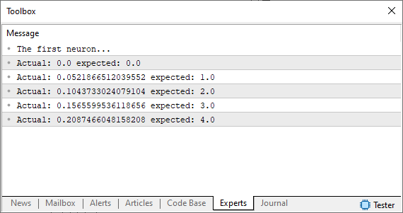
Note that we are using an assumption, which is the same random number that is not close to what we want or expect to get. How can we improve the situation? Okay, our basic neuron is on its way. Now we need to use the same principle as in the previous articles. In other words, we will define an error system so that the neuron knows where to move to find the most suitable equation. This is quite simple to do, as you can see in the code below.

//+------------------------------------------------------------------+
#property copyright "Daniel Jose"
//+------------------------------------------------------------------+
#define macroRandom (rand() / (double)SHORT_MAX)
//+------------------------------------------------------------------+
void OnStart()
{
    double Train[][2] {
                        {0, 0},
                        {1, 2},
                        {2, 4},
                        {3, 6},
                        {4, 8},
                      };
    double weight, fx, dx, x, err;
    const uint nTrain = Train.Size() / 2;

    Print("The first neuron...");
    MathSrand(512);
    weight = (double)macroRandom;
    err = 0;
        
    for (uint c = 0; c < nTrain; c++)
    {
        x = Train[c][0];
        fx = x * weight;
        Print("Actual: ", fx , " expected: ", x);
        dx = fx - Train[c][1];
        err += MathPow(dx, 2);
    }
    Print("Err: ", err / nTrain);
}
//+------------------------------------------------------------------+

Alright, when you run this code, you should see something similar to the image below.

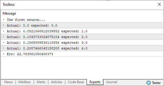
At this point, we're at a crossroads. This is the exact moment where, previously, we had to manually adjust values to minimize errors. If you're unsure what I mean, check out the previous articles for context. However, instead of making manual adjustments like before, this time, we'll let the computer do the work. Rather than finding the tangent line in the way we did previously, we'll approach it using the secant line. And this is where things start to get interesting - the machine will now begin to "go crazy" as it searches for the best possible fit. Sometimes, it will converge toward the correct solution, and at other times, it will diverge completely.

Our goal is to reduce the value of the variable 'err'. This is what drives the machine's unpredictable behavior. To understand this better, let's move on to a new topic.

Using the Secant Line

In the article "Neural Networks in Practice: The Secant Line" I briefly mentioned that the secant line plays a fundamental role in neural networks. There, I showed a diagram that you can review below.

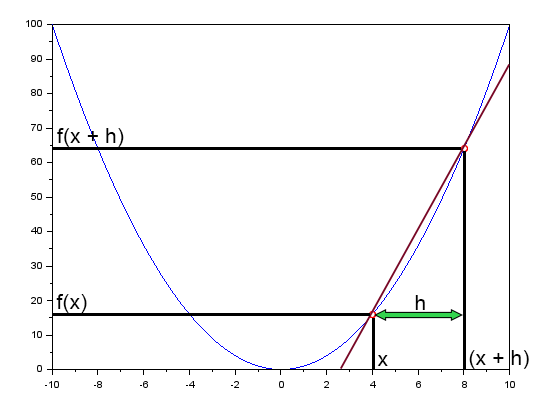
This diagram illustrates the error curve along with a straight line. This is the secant line. By simplifying the diagram and keeping only the secant line, we get the image shown next.

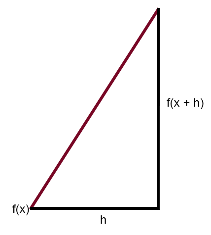
Now, if you modify this diagram so that the constant < h > equals zero, you get the following expression:

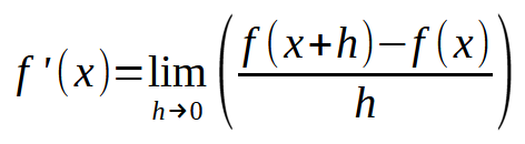
Here's where it gets exciting. The formula above is essentially the "magic formula" that allows a neural network to learn from its errors. By applying this equation, we can force the computer to find the best-fit line that represents the input data. This enables the machine to learn how to solve a given problem, whatever it may be. Regardless of what data you feed into the neural network, the underlying calculation remains the same. However, pay close attention: the key is choosing an appropriate value for < h >. If the value exceeds a certain limit, the machine will "go crazy" trying to find the best line equation. If the value is too small, the machine will spend a lot of time searching for the best-fitting equation, so a little common sense in this matter does not hurt. So, a bit of good judgment is needed here. Don't be overly demanding, but don't be too careless either. Find a balanced approach.

Now, how do we incorporate this into our neuron? Before making any changes, let’s do a small test first. Below is what our updated code should look like.

//+------------------------------------------------------------------+
#property copyright "Daniel Jose"
//+------------------------------------------------------------------+
#define macroRandom (rand() / (double)SHORT_MAX)
//+------------------------------------------------------------------+
double Train[][2] {
                    {0, 0},
                    {1, 2},
                    {2, 4},
                    {3, 6},
                    {4, 8},
                  };
//+------------------------------------------------------------------+
const uint nTrain = Train.Size() / 2;
const double eps = 1e-3;
//+------------------------------------------------------------------+
double Cost(const double w)
{
    double err;

    err = 0;
    for (uint c = 0; c < nTrain; c++)
        err += MathPow((Train[c][0] * w) - Train[c][1], 2);

    return err / nTrain;
}
//+------------------------------------------------------------------+
void OnStart()
{
    double weight;

    Print("The first neuron...");
    MathSrand(512);
    weight = (double)macroRandom;

    Print("Err: ", Cost(weight));
    Print("Err: ", Cost(weight + eps));
}
//+------------------------------------------------------------------+

Wow! Now this is starting to feel like a real program. When you run it, you should see something similar to the image below.

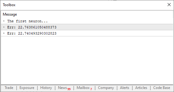
At this stage, what really matters is whether the error value is decreasing or increasing. The actual numerical value itself isn't important. Now, pay close attention: the variable 'eps' corresponds to the < h > we saw in the formula earlier. The closer this value gets to zero, the more each iteration will bring us closer to the tangent line. This happens because the secant line will start converging toward a limiting point. So, what's our next step? Something really simple: We need to create a loop that keeps reducing the error (or cost) with each iteration. Eventually, we'll reach a point where the error stops decreasing and begins to increase. At that exact moment, the program should detect this change and exit the loop. Otherwise, we'd risk entering an infinite loop. Alternatively, we can introduce another type of safeguard to prevent infinite loops. A common approach is to limit the number of iterations, ensuring the program stops if it fails to converge or if it starts "to go crazy". This instability could happen if the step size isn't well chosen. We'll explore this issue in more detail later. So for now, don't worry too much about it. That said, you’re free to fine-tune the program to push for the lowest possible cost value. It's entirely up to you when to end the loop. But to keep things simple, let's see what this looks like in practice. Check out the code below to understand how it works.

01. //+------------------------------------------------------------------+
02. #property copyright "Daniel Jose"
03. //+------------------------------------------------------------------+
04. #define macroRandom (rand() / (double)SHORT_MAX)
05. //+------------------------------------------------------------------+
06. double Train[][2] {
07.                     {0, 0},
08.                     {1, 2},
09.                     {2, 4},
10.                     {3, 6},
11.                     {4, 8},
12.                   };
13. //+------------------------------------------------------------------+
14. const uint nTrain = Train.Size() / 2;
15. const double eps = 1e-3;
16. //+------------------------------------------------------------------+
17. double Cost(const double w)
18. {
19.     double err;
20. 
21.     err = 0;
22.     for (uint c = 0; c < nTrain; c++)
23.         err += MathPow((Train[c][0] * w) - Train[c][1], 2);
24. 
25.     return err / nTrain;
26. }
27. //+------------------------------------------------------------------+
28. void OnStart()
29. {
30.     double weight, err;
31. 
32.     Print("The first neuron...");
33.     MathSrand(512);
34.     weight = (double)macroRandom;
35. 
36.     for(ulong c = 0; c < 10; c++)
37.     {
38.         err = ((Cost(weight + eps) - Cost(weight)) / eps);
39.         weight -= (err * eps);
40.         Print(c, "  -->  ", weight, " :: ", err);
41.     }
42.     Print("Weight: ", weight);
43. }
44. //+------------------------------------------------------------------+

When you run this code, you'll see something similar to the image below in the terminal.

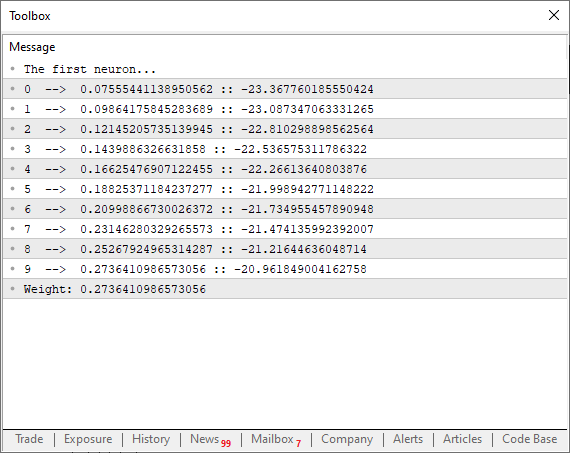
Now, take a closer look at an interesting detail. In line 38, we're performing the exact calculation we discussed earlier, where we force the secant line to search for the lowest possible limit, helping the function to converge. However, in line 39, notice that we're not just adjusting the curve point using the raw error or total cost value. But why? If we did that, the program would start jumping back and forth chaotically along the curve of the function. And that’s not what we want. We need the adjustments to be smooth and controlled. But why not use 'eps' to fine-tune the next point on the parabolic curve? Well, if we did, we'd have to constantly check whether the error is increasing or decreasing. Something that becomes completely unnecessary if we apply the factorization seen in line 39. This approach has another advantage, as it forces the neuron to converge faster at the beginning of the process. Then, as it gets closer to the ideal value, the decay curve smooths out, behaving like an inverted logarithmic decay function. And that's actually great! It means we'll reach an optimal error value much faster.

But we can make this code even better! We can add extra analysis tools to better understand what's happening. At the same time, we can introduce an additional test that allows the loop to terminate as soon as it reaches the minimum convergence point, even before hitting the maximum number of iterations. With that in mind, here’s the improved version of the code:

01. //+------------------------------------------------------------------+
02. #property copyright "Daniel Jose"
03. //+------------------------------------------------------------------+
04. #define macroRandom (rand() / (double)SHORT_MAX)
05. //+------------------------------------------------------------------+
06. double Train[][2] {
07.                     {0, 0},
08.                     {1, 2},
09.                     {2, 4},
10.                     {3, 6},
11.                     {4, 8},
12.                   };
13. //+------------------------------------------------------------------+
14. const uint nTrain = Train.Size() / 2;
15. const double eps = 1e-3;
16. //+------------------------------------------------------------------+
17. double Cost(const double w)
18. {
19.     double err;
20. 
21.     err = 0;
22.     for (uint c = 0; c < nTrain; c++)
23.         err += MathPow((Train[c][0] * w) - Train[c][1], 2);
24. 
25.     return err / nTrain;
26. }
27. //+------------------------------------------------------------------+
28. void OnStart()
29. {
30.     double weight, err, e1;
31.     int f = FileOpen("Cost.csv", FILE_COMMON | FILE_WRITE | FILE_CSV);
32. 
33.     Print("The first neuron...");
34.     MathSrand(512);
35.     weight = (double)macroRandom;
36. 
37.     for(ulong c = 0; (c < ULONG_MAX) && ((e1 = Cost(weight)) > eps); c++)
38.     {
39.         err = (Cost(weight + eps) - e1) / eps;
40.         weight -= (err * eps);
41.         if (f != INVALID_HANDLE)
42.             FileWriteString(f, StringFormat("%I64u;%f;%f\n", c, err, e1));
43.     }
44.     if (f != INVALID_HANDLE)
45.         FileClose(f);
46.     Print("Weight: ", weight);
47. }
48. //+------------------------------------------------------------------+

The beauty of this code is that it's incredibly fun to experiment with. It's designed so you can study, tweak, and play around with it. I decided to output the values not to the MetaTrader 5 terminal but to a file instead. This way, we can generate a graph and analyze what's happening more carefully. With the current configuration, the resulting graph looks like this:

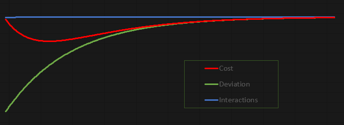
This graph was created in Excel, based on the values stored in the file generated by the neuron. Now, I'll admit that the way the file is created is a bit clunky. But since this is meant to be an educational and fun exercise, I don't see a problem with how we're transferring data to the file.

Final considerations

In this article, we built a basic neuron. Sure, it's simple, and some might think the code is too basic or pointless. But I want you, my reader, to play around with it and have fun. Don't be afraid to modify the code, understanding it fully is the goal. The code is attached so you can explore how a simple neuron works. Take your time reading this article. Try typing the code from scratch instead of copying and pasting it. Test each step until you reach the final version. Don't just copy my approach but build it in a way that makes sense to you. The key is to achieve the same end result: finding the correlation between the training data in the array. It's actually quite simple.

Since the code is included in the attachment, here are some interesting modifications you can try. Remember to calmly examine each modification. The first element is the training array, located in the sixth line of the application code. You can put different values there and have the neuron try to find a correlation between them.

Another very interesting point is the change in the value of the constant in line 15. Change it to a higher or lower value and observe the result the neuron reports at the end of its work. You will notice that lower values take longer to process, but the result will be much closer to the ideal value.

Another equally interesting point is in line 35, where we assign a weight that will fluctuate between zero and one. You can change it by multiplying the value returned by the macro. For example, try putting something like this in line 35.

weight = (double)macroRandom * 50;

You will notice that everything will be completely different, simply because you have changed the initial weight that the neuron starts with. And when you are completely sure of what is happening, you can change the code in line 34 to the one shown below.

MathSrand(GetTickCount()); 

You will notice that everything is much more interesting than many people think. But most importantly, you will begin to understand how a single neuron in a neural network can learn something. In the next article, we will turn this neuron into something even more interesting. So, before moving on to the next article, please study this code and experiment with it. Because this is just the beginning.