The Kalman Filter for Forex Mean-Reversion Strategies

Introduction

The Kalman filter is a recursive algorithm used in algorithmic trading to estimate the true state of a financial time series by filtering out noise from price movements. It dynamically updates predictions based on new market data, making it valuable for adaptive strategies like mean reversion. This article first introduces the Kalman filter, covering its calculation and implementation. Next, we apply the filter to a classic mean-reversion forex strategy as an example. Finally, we conduct various statistical analyses by comparing the filter with a moving average across different forex pairs.

The Kalman Filter

The Kalman filter, introduced by Rudolf E. Kalman in 1960, is an optimal recursive estimator used for tracking and predicting dynamic systems. Originally developed for aerospace and control systems, it has been widely applied in finance, robotics, and signal processing. The filter operates in two steps: a prediction step, where it estimates the system’s next state, and an update step, where it refines the estimate based on new observations while minimizing noise. 

In the field of algorithmic trading, one can simply see it as a common regime filter that traders normally use, akin to moving average or linear regression models. The Kalman filter adapts dynamically to new data, reduces noise, and efficiently updates estimates in real-time, making it effective for detecting market regime shifts. However, it assumes linear dynamics, requires careful parameter tuning, may lag in detecting abrupt changes, and is computationally more complex than simpler filters like moving averages.

Some common usages for using the Kalman filter in algorithmic trading:

• Mean Reversion Trading: Using current price compared to estimated price as an entry filter.
• Pairs Trading: Dynamically estimates the spread between correlated assets and adjusts hedge ratios based on changing market conditions.
• Trend Following: Filters short-term noise to detect long-term price trends more accurately.
• Volatility Estimation: Provides adaptive estimates of market volatility for risk management and position sizing.

The formula of calculating the Kalman filter value is as follows:

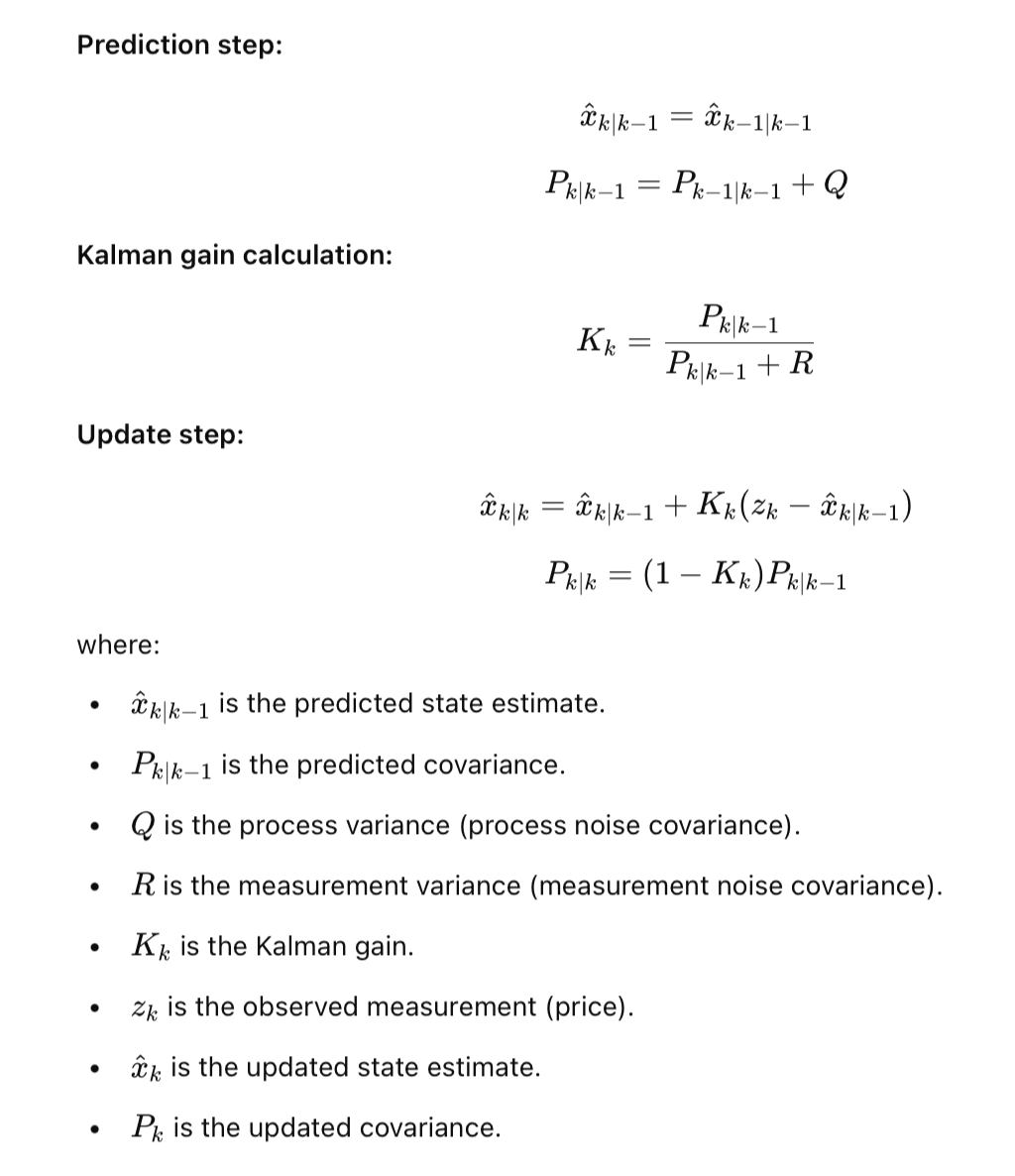
To understand the complex formula in a simple way, let us turn to a visualization example.

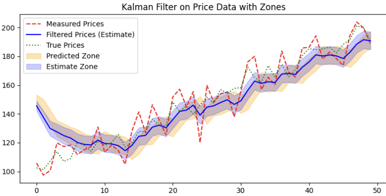
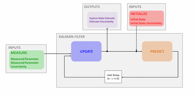
The Kalman filter works by updating its estimate of the true price based on noisy measurements and predictions. It is usually obtained in three steps:

1. Prediction: The filter starts with an initial guess for the price (predicted price) and its uncertainty (predicted covariance). This is shown by the orange Predicted Zone—the range within which the filter expects the true price to be, considering both the previous estimate and the process noise.

2. Update: When new price data (measured prices) is available, the Kalman filter compares it to the predicted price. It then calculates something called the Kalman Gain (purple line) to decide how much weight to give the new measurement versus the prediction. If the measurement is very noisy, the filter trusts its prediction more. 

3. Estimate: The filter updates the predicted price by incorporating the new measurement. The updated price (shown by the blue Estimate Zone) has a reduced uncertainty compared to the prediction. This zone shrinks as the filter refines its estimate. 

Here, the prediction uncertainty is defined by covariance between the measurement and prediction. A larger covariance means a less confident estimate, while a smaller covariance means the filter is more certain about its estimate. If the measurement is reliable, the Kalman gain is high, and the filter trusts the new data more (shrinking uncertainty). If the measurement is noisy, the gain is lower, and the filter relies more on the previous prediction.

The nosiness is defined by the variance, namely the measurement variance and process variance. They don't self-adjust like covariance, they are determined from the start based on how smooth you want your Kalman filter to be.

Here are some examples of how the variances affect the smoothness of the curve:

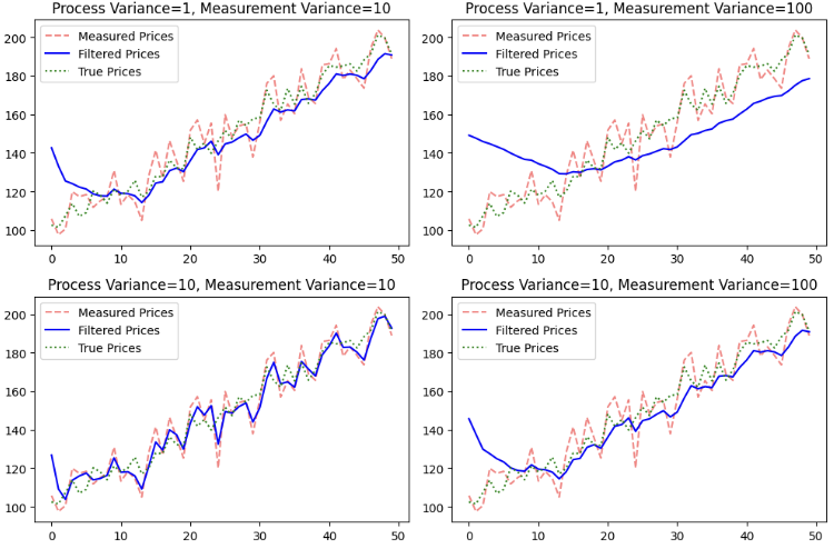
In general, process variance (Q) represents how much the model expects the true state to change over time, while measurement variance (R) reflects the confidence in the observed data. Higher Q makes the filter more responsive to sudden changes, but increases volatility. Higher R smooths predictions by trusting past estimates more, at the cost of delayed adjustments. Low Q and moderate R yield stable predictions, while high Q and low R make the filter more reactive but noisier.

Coding the Strategy

Mean-reversion strategies often follow the approach of buying when oversold, selling when overbought, and exiting when the price reverts to the mean. This strategy is based on the assumption that price data is generally stable and doesn't tend to reach extreme levels. When the price is at one extreme, it is expected to eventually return to the equilibrium point. This theory holds especially true for semi-stationary data like forex, where mean-reversion strategies have been profitable over the years.

We will quantify our approach using 100-period Bollinger Bands with a 2.0 deviation. The detailed plan is as follows:

• Buy when the last close price is lower than the lower band.
• Sell when the last close price is higher than the upper band.
• Close the position whenever the price crosses the middle band.
• Only one position at a time to avoid over-trading.
• Set the stop loss gap at 1% of price to avoid fat tail risk that is common for mean-reversion strategies.

We plan to trade forex pairs on the 15-minute timeframe, a common timeframe that provides enough trades while ensuring decent trade quality.

We always start by defining the necessary functions first, as this makes the trade logic coding easier later on. In this case, we only need to code the buy and sell functions as follows:

#include <Trade/Trade.mqh>
CTrade trade;
//+------------------------------------------------------------------+
//| Buy Function                                                     |
//+------------------------------------------------------------------+
void executeBuy(string symbol) {
       double ask = SymbolInfoDouble(symbol, SYMBOL_ASK);
       double lots=0.01;
       double sl = ask*(1-0.01);
       trade.Buy(lots,symbol,ask,sl);
}

//+------------------------------------------------------------------+
//| Sell Function                                                    |
//+------------------------------------------------------------------+
void executeSell(string symbol) {      
       double bid = SymbolInfoDouble(symbol, SYMBOL_BID);
       double lots=0.01;
       double sl = bid*(1+0.01);
       trade.Sell(lots,symbol,bid,sl);     
}

Then, we initialize the global variables and the initializer here. This initializes the magic number for the expert advisor, as well as the Bollinger Band's handle that we will use later.

input int Magic = 0;
input int bbPeriod = 100;
input double d = 2.0;

int barsTotal = 0;
int handleMa;

//+------------------------------------------------------------------+
//| Initialization                                                   |
//+------------------------------------------------------------------+
int OnInit()
{   handleBb = iBands(_Symbol,PERIOD_CURRENT,bbPeriod,0,d,PRICE_CLOSE);  
    trade.SetExpertMagicNumber(Magic);
    return INIT_SUCCEEDED;
}

Finally, in the OnTick() function, we use this to ensure that we only process the trade logic every bar instead of every tick:

int bars = iBars(_Symbol,PERIOD_CURRENT);
  
if (barsTotal!= bars){
   barsTotal = bars;

We obtain the current values of the Bollinger Bands by creating buffer arrays that can store the current values by copying from the handle.

double bbLower[], bbUpper[], bbMiddle[];
CopyBuffer(handleBb,UPPER_BAND,1,1,bbUpper);
CopyBuffer(handleBb,LOWER_BAND,1,1,bbLower);
CopyBuffer(handleBb,0,1,1,bbMiddle);

This check loops through all the current opened positions in the trading account to check whether the position is opened by this specific EA. If there is already a position opened by this EA, we set the NotInPosition variable to false. For every opened position that have reverted back to the middle band, we close it.

bool NotInPosition = true;
for(int i = 0; i<PositionsTotal(); i++){
    ulong pos = PositionGetTicket(i);
    string symboll = PositionGetSymbol(i);
    if(PositionGetInteger(POSITION_MAGIC) == Magic&&symboll== _Symbol){
       NotInPosition = false;
       if((PositionGetInteger(POSITION_TYPE) == POSITION_TYPE_BUY&&price>bbMiddle[0])
       ||(PositionGetInteger(POSITION_TYPE) == POSITION_TYPE_SELL&&price<bbMiddle[0]))trade.PositionClose(pos);  
  }
}  

The final trade logic will be carried out like this:

if(price<bbLower[0]&&NotInPosition) executeBuy(_Symbol);
if(price>bbUpper[0]&&NotInPosition) executeSell(_Symbol);

Compile the EA and head to strategy tester visualizer to see if the EA is working as expected.

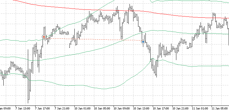
A typical trade in the visualizer should look like this:

We then go back to MetaEditor and code the regime filters.

First, for the 500-EMA, we want the mean-reversion strategy to align with the trend when entering, as an additional confirmation. We add these lines to the original EA:

int handleMa;
handleMa = iMA(_Symbol,PERIOD_CURRENT,maPeriod,0,MODE_EMA,PRICE_CLOSE);
 
double ma[];
CopyBuffer(handleMa,0,1,1,ma);
    
if(price<bbLower[0]&&price>ma[0]&&NotInPosition) executeBuy(_Symbol);
if(price>bbUpper[0]&&price<ma[0]&&NotInPosition) executeSell(_Symbol);

 After that, we code the function for getting the Kalman filter value:

//+------------------------------------------------------------------+
//| Kalman Filter Function                                           |
//+------------------------------------------------------------------+
double KalmanFilter(double price,double measurement_variance,double process_variance)
{
    // Prediction step (state does not change)
    double predicted_state = prev_state;
    double predicted_covariance = prev_covariance + process_variance;

    // Kalman gain calculation
    double kalman_gain = predicted_covariance / (predicted_covariance + measurement_variance);

    // Update step (incorporate new price observation)
    double updated_state = predicted_state + kalman_gain * (price - predicted_state);
    double updated_covariance = (1 - kalman_gain) * predicted_covariance;

    // Store updated values for next iteration
    prev_state = updated_state;
    prev_covariance = updated_covariance;

    return updated_state;
}

The function follows the recursive procedure like this diagram:

To implement the Kalman regime filter in the EA, we add these lines to the OnTick() function:

double kalman = KalmanFilter(price,mv,pv);
if(price<bbLower[0]&&price>kalman&&NotInPosition) executeBuy(_Symbol);
if(price>bbUpper[0]&&price<kalman&&NotInPosition) executeSell(_Symbol);

The Kalman filter works by continuously updating its estimate of the true price, smoothing out noise, and adapting to price movements over time. It essentially acts as a price predictor. When the price falls below the lower band of the Bollinger Bands, it signals that the market is oversold and is expected to revert to the mean. Here, we use the Kalman filter as a confirmation of the reversal. In the oversold scenario, if the price is higher than the Kalman estimate, it suggests that the price has already shown signs of potential upward movement. In the sell scenario, the reverse is true.

However, while the moving average is also a common regime filter, its purpose is slightly different from that of the Kalman filter. Moving averages serve as a trend indicator, with the position of the price relative to the MA signaling the current trend direction.

The full code is as follows:

#include <Trade/Trade.mqh>
CTrade trade;

input double mv = 10;
input double pv = 1.0;
input int Magic = 0;
input int bbPeriod = 100;
input double d = 2.0;
input int maPeriod = 500;

double prev_state;       // Previous estimated price
double prev_covariance = 1;  // Previous covariance (uncertainty)
int barsTotal = 0;
int handleMa;
int handleBb;

//+------------------------------------------------------------------+
//| Initialization                                                   |
//+------------------------------------------------------------------+
int OnInit()
{   handleMa = iMA(_Symbol,PERIOD_CURRENT,maPeriod,0,MODE_EMA,PRICE_CLOSE);
    handleBb = iBands(_Symbol,PERIOD_CURRENT,bbPeriod,0,d,PRICE_CLOSE);
    prev_state = iClose(_Symbol,PERIOD_CURRENT,1);  
    trade.SetExpertMagicNumber(Magic);
    return INIT_SUCCEEDED;
}

//+------------------------------------------------------------------+
//| Deinitializer function                                           |
//+------------------------------------------------------------------+
void OnDeinit(const int reason)
  {
  }

//+------------------------------------------------------------------+
//| OnTick Function                                                  |
//+------------------------------------------------------------------+
void OnTick()
{
  int bars = iBars(_Symbol,PERIOD_CURRENT);
  
  if (barsTotal!= bars){
     barsTotal = bars;
     bool NotInPosition = true;
     double price = iClose(_Symbol,PERIOD_CURRENT,1); 
     double bbLower[], bbUpper[], bbMiddle[];
     double ma[];
     double kalman = KalmanFilter(price,mv,pv);
     
     CopyBuffer(handleMa,0,1,1,ma);
     CopyBuffer(handleBb,UPPER_BAND,1,1,bbUpper);
     CopyBuffer(handleBb,LOWER_BAND,1,1,bbLower);
     CopyBuffer(handleBb,0,1,1,bbMiddle);
     
     for(int i = 0; i<PositionsTotal(); i++){
         ulong pos = PositionGetTicket(i);
         string symboll = PositionGetSymbol(i);
         if(PositionGetInteger(POSITION_MAGIC) == Magic&&symboll== _Symbol){
            NotInPosition = false;
            if((PositionGetInteger(POSITION_TYPE) == POSITION_TYPE_BUY&&price>bbMiddle[0])
            ||(PositionGetInteger(POSITION_TYPE) == POSITION_TYPE_SELL&&price<bbMiddle[0]))trade.PositionClose(pos);  
      }
    }  
    
     if(price<bbLower[0]&&price>kalman&&NotInPosition) executeBuy(_Symbol);
     if(price>bbUpper[0]&&price<kalman&&NotInPosition) executeSell(_Symbol);
    }
}

//+------------------------------------------------------------------+
//| Kalman Filter Function                                           |
//+------------------------------------------------------------------+
double KalmanFilter(double price,double measurement_variance,double process_variance)
{
    // Prediction step (state does not change)
    double predicted_state = prev_state;
    double predicted_covariance = prev_covariance + process_variance;

    // Kalman gain calculation
    double kalman_gain = predicted_covariance / (predicted_covariance + measurement_variance);

    // Update step (incorporate new price observation)
    double updated_state = predicted_state + kalman_gain * (price - predicted_state);
    double updated_covariance = (1 - kalman_gain) * predicted_covariance;

    // Store updated values for next iteration
    prev_state = updated_state;
    prev_covariance = updated_covariance;

    return updated_state;
}

//+------------------------------------------------------------------+
//| Buy Function                                                     |
//+------------------------------------------------------------------+
void executeBuy(string symbol) {
       double ask = SymbolInfoDouble(symbol, SYMBOL_ASK);
       double lots=0.01;
       double sl = ask*(1-0.01);
       trade.Buy(lots,symbol,ask,sl);
}

//+------------------------------------------------------------------+
//| Sell Function                                                    |
//+------------------------------------------------------------------+
void executeSell(string symbol) {      
       double bid = SymbolInfoDouble(symbol, SYMBOL_BID);
       double lots=0.01;
       double sl = bid*(1+0.01);
       trade.Sell(lots,symbol,bid,sl);     
} 

To change the regime filter, simply adjust the final buy/sell criteria.

Statistical Analysis

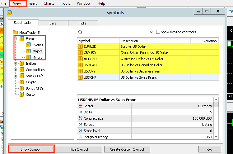
Compile the EA and go to the MetaTrader 5 terminal, on the top left, click View->Symbols->Forex and select "Show Symbol" for all major pairs and minor pairs. This puts them in your market watch list for later market scanning.

Then, we go to the Market Scanner in the Strategy Tester section and backtest the strategy using data from the past 3 years. This will help us get a sense of whether the regime filters improve profitability for the majority of the forex pairs we might be trading.

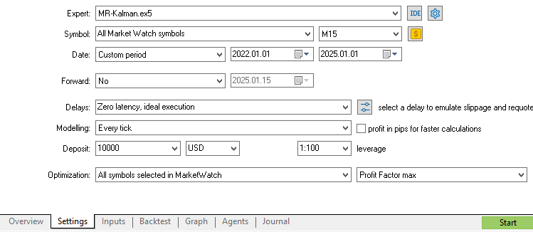
Of course, the number of filtered trades depends on the parameters of the indicators. In this study, we use commonly applied parameter values that filter a similar number of trades: a 500-period exponential moving average and a measurement variance of 10 and process variance of 1 for the Kalman filter. Readers are encouraged to fine-tune the parameters for the most effective results.

We first test the result with no regime filters involved as a baseline. We expect that, on average, the EA with regime filters should outperform the majority of the baseline results.

The result of the top-performing forex pairs shows something like this:

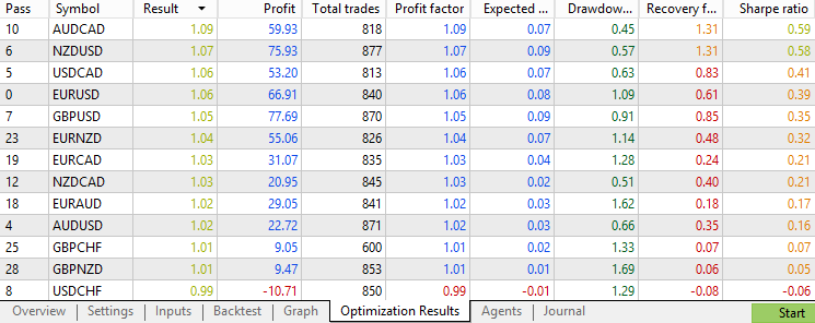
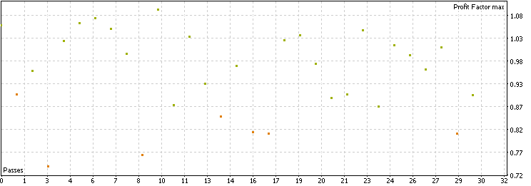
We see that, on average, the strategy executes 800+ trades in the past 3 years for each pair, providing enough samples to imply generality in the conclusions. The distribution is mostly scattered around a 0.8–1.1 profit factor, which is decent, but no pairs exceed the 1.1 profit factor or 1 Sharpe ratio mark. Overall, the raw strategy works across many forex pairs in recent years, but the profitability isn't particularly impressive. Keep this in mind as we compare it with the performance when filters are applied.

Next, we backtest the strategy with the moving average filter involved. Here are the results:

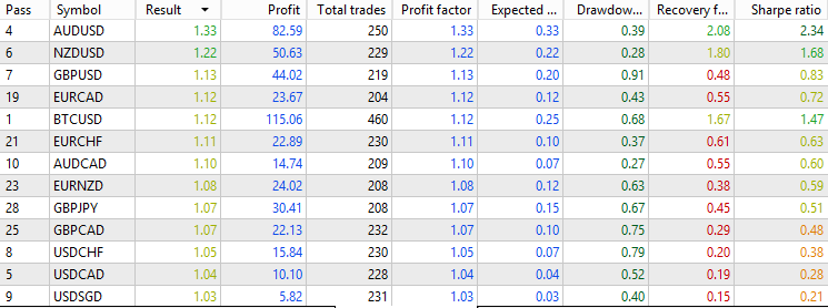
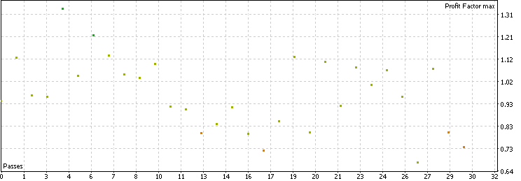
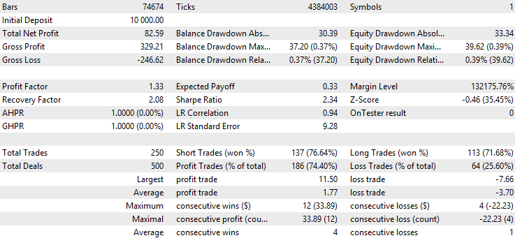
We see that, by using the moving average filter, we filtered out about 70% of the original trades, leaving approximately 250 trades for each pair. Additionally, the filtered trades are, on average, of higher quality compared to the baseline. Most forex pairs hover between a 0.9 and 1.2 profit factor, with the best-performing pair having a 1.33 profit factor and a 2.34 Sharpe ratio. This suggests that using the moving average as a filter has overall improved the profitability of this classic mean-reversion strategy.

Now, let's address the elephant in the room and see how the strategy performs with the Kalman filter.

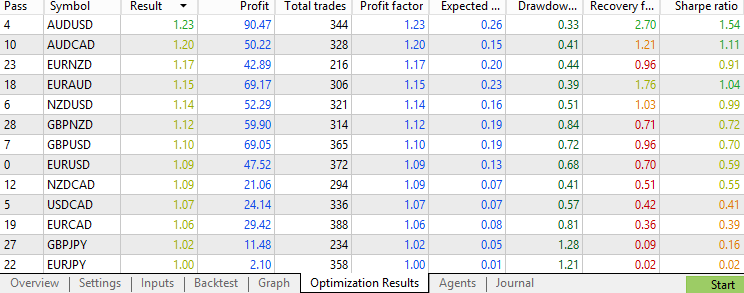
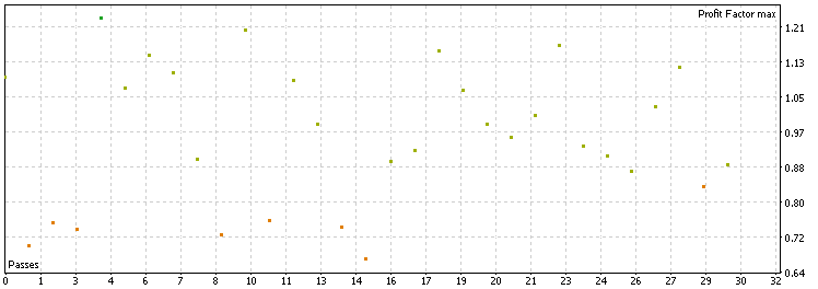
The Kalman filter filtered out about 60% of the original trades, leaving about 350 trades for each pair. From the distribution, we see that most profit factors stay between 0.85 and 1.2, which is similar to the moving average performance and better than the baseline performance. Moreover, considering the overall number of forex pairs with a 1.0+ profit factor and 1.2+ profit factor, we may conclude that both the moving average and the Kalman filter are similar in terms of improving the average trade quality for this strategy. The Kalman filter is not superior to the moving average in this scenario, suggesting that complexity does not always result in better performance.

We mentioned that the use of the Kalman filter differs slightly from the use of the moving average in terms of filtering logic. However, in this case, they seem to perform similarly in terms of filtering out bad trades. To investigate whether they are filtering similar trades, we will analyze the differences between their filtered trades to determine whether the effect of the Kalman filter is merely the same as the EMA.

For reference, we will choose the AUDUSD forex pair, as it has been the best performing pair across all two conditions mentioned above.

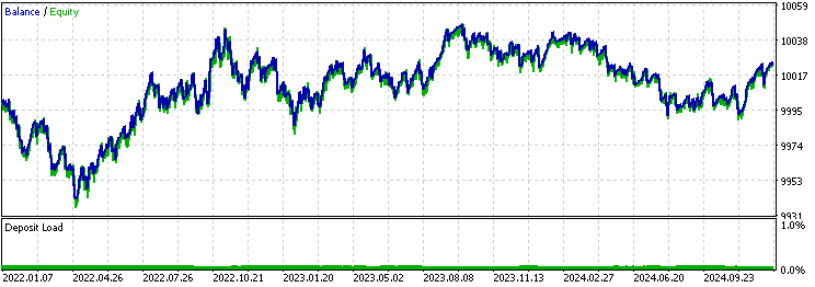
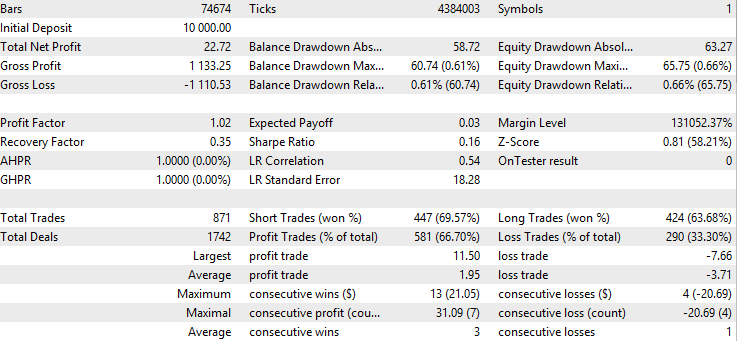
The backtest result of the baseline:

The backtest result of the exponential moving average filter:

The result of the Kalman filter:

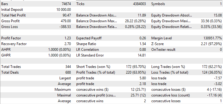
The first thing we can notice is that the win rate of the moving average version is significantly higher than the baseline or the Kalman version, while its average profit is lower and its average loss is higher than the others. This already suggests that the moving average version is taking very different trades than the Kalman version. To further investigate, we obtain the backtest excel report by right-clicking on the backtest result page:

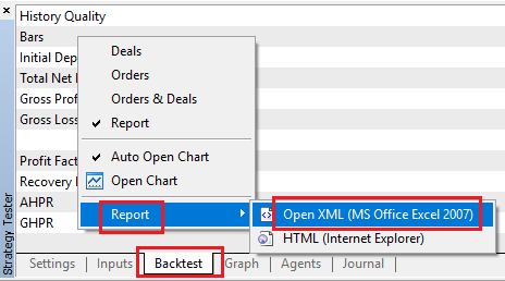
For each report, we note the row number of the "Deals" sign:

Next, we go into Python or Jupyter Notebook. We copy and paste the following code, change the skiprow number to each Excel report's "Deals" row number, and we’re done.

import pandas as pd
import matplotlib.pyplot as plt
from matplotlib_venn import venn3
df1 = pd.read_excel("baseline.xlsx", skiprows=1805)
df2 = pd.read_excel("ma.xlsx", skiprows =563 )
df3 = pd.read_excel("kalman.xlsx",skiprows = 751)
df1 = df1[['Time']][1:-1]
df1 = df1[df1.index % 2 == 0]  # Filter for rows with odd indices
df2 = df2[['Time']][1:-1]
df2 = df2[df2.index % 2 == 0]
df3 = df3[['Time']][1:-1]
df3 = df3[df3.index % 2 == 0]

# Convert "Time" columns to datetime
df1['Time'] = pd.to_datetime(df1['Time'])
df2['Time'] = pd.to_datetime(df2['Time'])
df3['Time'] = pd.to_datetime(df3['Time'])

# Find intersections
set1 = set(df1['Time'])
set2 = set(df2['Time'])
set3 = set(df3['Time'])

# Create the Venn diagram
venn_labels = {
    '100': len(set1 - set2 - set3),  # Only in df1
    '010': len(set2 - set1 - set3),  # Only in df2
    '001': len(set3 - set1 - set2),  # Only in df3
    '110': len(set1 & set2 - set3),  # In df1 and df2
    '011': len(set2 & set3 - set1),  # In df2 and df3
    '101': len(set1 & set3 - set2),  # In df1 and df3
    '111': len(set1 & set2 & set3)   # In all three
}

# Plot the Venn diagram
plt.figure(figsize=(8, 8))
venn3(subsets=venn_labels, set_labels=('Baseline', 'EMA', 'Kalman'))
plt.title("Venn Diagram of Time Overlap")
plt.show()

The logic of this code is essentially that we store the position exit times into three dataframes for each version by skipping rows and selecting rows with even indices. Then, we store each data frame into a set and obtain the Venn diagram by comparing whether the times overlap. The graph will show the number of trades in each region, separated by different colors. Note that even the baseline won't contain all the trades that the EMA and Kalman versions have because we set the strategy to trade only one at a time, which causes it to miss out on some trades that the other versions have.

Here’s the output Venn diagram:

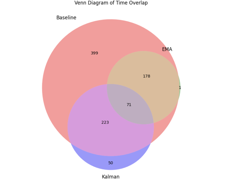
Observing the area where the Kalman and MA overlap, we find that among the hundreds of trades each version took, only 71 trades were the same. This suggests that the filter effects of these two are very dissimilar, despite filtering out a similar number of trades from the original strategy. This further emphasizes the importance of studying and utilizing the Kalman filter, as it provides a unique filtering option that differs from common trend filters.

Conclusion

In this article, we introduced an advanced recursive algorithm for algorithmic trading called the Kalman filter. We started by explaining its mechanisms and implementations, providing visualizations and formulas. Then, we walked through the entire process of developing a forex mean-reversion strategy and implementing the Kalman filter in MQL5. Finally, we conducted various statistical analyses, including market scanning, backtesting, and overlapping comparisons, to evaluate its filtering ability in comparison to the moving average and baseline.

In actual trading, the Kalman filter is widely used by top quantitative trading institutions but remains lesser known in the retail trading space. This article aims to provide insights and practical implementation for the MQL5 community, offering an approach to evaluate the filtering ability of the Kalman filter, so it can be better integrated into future strategy development. Readers are encouraged to experiment with this framework themselves and incorporate it into their own trading arsenal.

File Table

File Name	File Usage
Kalman visualizations.ipynb	The python code for visualizations used in this article
MR-Kalman.mq5	The expert advisor code