Frequency domain representations of time series: The Power Spectrum

Introduction

Price quotes we observe on charts represent data spread out across time. The series of prices is said to be in the time domain . But this is not the only way to express this information . Displaying the data in different domains can reveal interesting characteristics about the series that may not be apparent when conducting analysis exclusively in the time domain. In this article  we will discuss some of the useful perspectives to be gained by analyzing time series in the frequency domain using  the discrete fourier transform (dft). We focus on the analysis of power spectra  by providing  practical examples of how to calculate and recognise time series features as revealed by this method of analysis. We will also briefly discuss important preprocessing techniques that should be applied before applying the discrete fourier transform.

The discrete fourier transform

Before demonstrating the methods of power spectrum analysis we first have to understand what the power spectrum is. Analysis of the power spectra of time series  falls under the broad topic of signal processing.  In the article Technical Indicators and Digital Filters the author shows how any complicated series can be brocken up into common sine and cosine wave forms. This makes it possible to reduce a complex process into simple components. What makes all this possible is the frequency domain representation chosen. This refers to the basis of representation which is the collection of functions that are used to reproduce a time series.

One of the most commonly applied frequency domain representations of time series is the discrete fourier transform. It uses as its basis the sine and cosine waves that cover one cycle for the extent of a series. Its most invaluable characteristic is that any time series outlined in this form is always uniquely defined, that is no two series will have similar representations in the frequency domain. A power spectrum is a representation of how much power, or energy, a signal has at different frequencies. In the context of a time series data, the power spectrum provides information about the distribution of energy across the different frequencies that make up the time series.

Computing the discrete fourier transform

To convert any series to the frequency domain using  the dft , the formula below is applied.

Where each term is a complex number and x is the raw data series. Each term represents a periodic component that repeats exactly j times across the extent of the range of values. The fast fourier transform is an algorithm that accelerates the computation of discrete fourier transformations. It recursively splits a series in half, transforming each half, then eventually combining the results.

The Power Spectrum

By applying some basic math we can calculate the amount of energy due to a frequency component . Plotting a complex number on a cartesian plane , where the real part is plotted on the x axis  and the imaginary part on the y axis we can apply  Pythagoras' theorem which stipulates that the absoute value is the square root of the sum of the squares of both real and imaginary parts. Therefore the energy due to a certain frequency is the square of its absolute value. The power is calculated by dividing its squared absolute value by the square of the number of values in the time domain series.

But before we apply the raw dft calculation to a series we have to go through a few preprocessing steps to get an accurate estimate of the power at a particular frequency. This is necessary because the dft operates on finite-length segments of data and it assumes that the input signal is periodic, which can lead to spectral leakage and other distortions if the values do not meet this assumption. To mitigate these problems data windowing is applied.

Data Windowing

Data windowing refers to the process of multiplying a time series by a window function, which is a mathematical function that assigns weights to different points in the time series. Data windowing is an important step in preparing time series data for analysis using the discrete fourier transform.

When we analyze time series data using the dft, we divide the data into smaller segments. If we don't add a frame (in this case, a window function) around each segment, we might miss some important information and our analysis will be incomplete. Data windowing tapers the ends of the time series, reducing the abrupt transitions at the boundaries of the dft window. The tapering function is typically designed to smoothly taper the signal to zero at the edges of the window, which reduces the amplitude of any spectral components near the edge of the window.

Important as this process may be it does introduce some problems that can cause distortion or changes in the original shape of the data. Most of these problems can be eliminated or minimized by centering the series prior to applying a windowing function to the raw series.  When a time series is centered, its mean value is subtracted from every data point in the series, resulting in a new series with a zero mean.

There are many windowing functions available,such as the rectangular window, the Hamming window, Hanning window, the Blackman window and the Kaiser window, each has its own unique properties and use cases. In this text we will use the Welch data window, which is another popular windowing method.  
    
The Welch data window is given by the formula below.

Each value of the original time series must be multiplied by the a corresponding m(i).

In order to center the values the weighted average of the series is calculated using the window function. This average is then subtracted from each point in the series  before application of the window itself.

Smoothing the power spectrum

The discrete power spectrum can be difficult to interpret as there are usually a lot of narrow peaks, jutting up all over the place. To get a better sense of what is going on it may be necessary to employ some smoothing . The Saviztky Golay filter is usually the favoured choice in these applications. Its filtering function is defined by two parameters , the half length and the degree of polynomials. The half length specifies the number of values adjacent ( before and after ) a value being filtered. The degrees define the degree of polynomial to be fitted to the current value and its adjacent values.

The CSpectrum Class

In this section we present a class that enables easy analysis of series in mql5. One of the highlights of the class includes the implementation of a plot method that facilitates the display of various spectral plots using a few lines of code.

The whole class is defined below.

//+------------------------------------------------------------------+
//|                                                     Spectrum.mqh |
//|                        Copyright 2023, MetaQuotes Software Corp. |
//|                                             https://www.mql5.com |
//+------------------------------------------------------------------+
#property copyright "Copyright 2023, MetaQuotes Software Corp."
#property link      "https://www.mql5.com"
#include<Math\Stat\Math.mqh>
#include<Math\Alglib\fasttransforms.mqh>
#include<Graphics\Graphic.mqh>

enum ENUM_SPECTRUM_PLOT
  {
   PLOT_POWER_SPECTRUM=0,//PowerSpectrum
   PLOT_FILTERED_POWER_SPECTRUM,//FilteredPowerSpectrum
   PLOT_CUMULATIVE_SPECTRUM_DEVIATION//CumulativeSpectrumDeviation
  };

//+------------------------------------------------------------------+
//|                                                                  |
//+------------------------------------------------------------------+
class CSpectrumAnalysis
  {
private:
   bool              m_window,m_initialized;
   int               m_n,m_cases;
   complex           m_dft[];
   double            m_real[];
   double            m_win,m_win2;
   double            m_wsq;
   double            m_wsum,m_dsum;
   int               m_window_size,m_poly_order;
   void              savgol(double &data[], double&out[], int window_size, int poly_order);
public:
   //---constructor
                     CSpectrumAnalysis(const bool window,double &in_series[]);
   //---destructor
                    ~CSpectrumAnalysis(void)
     {
      if(m_n)
        {
         ArrayFree(m_dft);
         ArrayFree(m_real);
        }
     }
   bool              PowerSpectrum(double &out_p[]);
   bool              CumulativePowerSpectrum(double & out_cp[]);
   double            CumulativeSpectrumDeviation(double &out_csd[]);
   void              Plot(ENUM_SPECTRUM_PLOT plot_series,int window_size=5, int poly_order=2, color line_color=clrBlue, int display_time_seconds=30, int size_x=750, int size_y=400);
  };

To use it a user calls the parametric constructor by passing it two parameters. The first parameter specifies whether to apply a windowing function to the data. It should be noted that by  opting to apply a windowing function, centering of the series is also undertaken. The second parameter to the constructor is an array that contains the raw values to be analyzed.

The fourier transformation is done in the constructor and the complex values associated with the spectrum are stored in the dft array.

void CSpectrumAnalysis::CSpectrumAnalysis(const bool apply_window,double &in_series[])
  {
   int n=ArraySize(in_series);

   m_initialized=false;

   if(n<=0)
      return;

   m_cases=(n/2)+1;
   m_n=n;

   m_window=apply_window;

   ArrayResize(m_real,n);

   if(m_window)
     {
      m_wsum=m_dsum=m_wsq=0;
      for(int i=0; i<n; i++)
        {
         m_win=(i-0.5*(n-1))/(0.5*(n+1));
         m_win=1.0-m_win*m_win;
         m_wsum+=m_win;
         m_dsum+=m_win*in_series[i];
         m_wsq+=m_win*m_win;
        }
      m_dsum/=m_wsum;
      m_wsq=1.0/sqrt(n*m_wsq);
     }
   else
     {
      m_dsum=0;
      m_wsq=1.0;
     }


   for(int i=0; i<n; i++)
     {
      if(m_window)
        {
         m_win=(i-0.5*(n-1))/(0.5*(n+1));
         m_win=1.0-m_win*m_win;
        }
      else
         m_win=1.0;
      m_win*=m_wsq;
      m_real[i]=m_win*(in_series[i]-m_dsum);
     }
   CFastFourierTransform::FFTR1D(m_real,n,m_dft);

   m_initialized=true;

  }

In order to calculate and get the values of the power spectrum , cumulative power spectrum and also the cumulative spectrum deviation the class provides the methods PowerSpectrum(), CumulativePowerSpectrum() and CumulativeSpectrumDeviation() respectively. Each method requires a single array parameter, where the corresponding values will be copied.

//+------------------------------------------------------------------+
//|                                                                  |
//+------------------------------------------------------------------+
bool CSpectrumAnalysis::PowerSpectrum(double &out_p[])
  {
   if(!m_initialized)
      return false;

   ArrayResize(out_p,m_cases);

   for(int i=0; i<m_cases; i++)
     {
      out_p[i]=m_dft[i].re*m_dft[i].re + m_dft[i].im*m_dft[i].im;
      if(i && (i<(m_cases-1)))
         out_p[i]*=2;
     }

   return true;
  }
//+------------------------------------------------------------------+
//|                                                                  |
//+------------------------------------------------------------------+
bool CSpectrumAnalysis::CumulativePowerSpectrum(double &out_cp[])
  {
   if(!m_initialized)
      return false;

   double out_p[];

   ArrayResize(out_p,m_cases);
   ArrayResize(out_cp,m_cases);

   for(int i=0; i<m_cases; i++)
     {
      out_p[i]=m_dft[i].re*m_dft[i].re + m_dft[i].im*m_dft[i].im;
      if(i && (i<(m_cases-1)))
         out_p[i]*=2;
     }

   for(int i=0; i<m_cases; i++)
     {
      out_cp[i]=0;
      for(int j=i; j>=1; j--)
         out_cp[i]+=out_p[j];
     }

   ArrayFree(out_p);

   return true;

  }
//+------------------------------------------------------------------+
//|                                                                  |
//+------------------------------------------------------------------+
double CSpectrumAnalysis::CumulativeSpectrumDeviation(double &out_csd[])
  {
   if(!m_initialized)
      return 0;

   ArrayResize(out_csd,m_cases);

   double sum=0;
   for(int i=0; i<m_cases; i++)
     {
      out_csd[i]=m_dft[i].re*m_dft[i].re + m_dft[i].im*m_dft[i].im;
      if(i==(m_cases-1))
         out_csd[i]*=0.5;
      sum+=out_csd[i];
     }
   double sfac=1.0/sum;
   double nfac=1.0/(m_cases-1);
   double dmax=sum=0;

   for(int i=1; i<m_cases-1; i++)
     {
      sum+=out_csd[i];
      out_csd[i]=sum*sfac - i*nfac;
      if(MathAbs(out_csd[i])>dmax)
         dmax=MathAbs(out_csd[i]);
     }
   out_csd[0]=out_csd[m_cases-1]=0;

   return dmax;
  }

The last method of note is the Plot() function. With it a user can quickly display one graphical plot from a choice of three options defined by the ENUM_SPECTRUM_PLOT enumeration. The second  and third parameters of the Plot() method define the smoothing parameters applied to the Savitzky-Golay filter when plotting the filtered cumulative power spectrum. When other plots are selected these parameters have no effect. The rest of the parameters of Plot() control the color of the line plot, the amount of time the graphic will be displayed in seconds and size of the plot respectively.

void CSpectrumAnalysis::Plot(ENUM_SPECTRUM_PLOT plot_series,int windowsize=5, int polyorder=2,color line_color=clrBlue, int display_time_seconds=30, int size_x=750, int size_y=400)
  {
   double x[],y[];
   bool calculated=false;

   string header="";

   switch(plot_series)
     {
      case PLOT_POWER_SPECTRUM:
         ArrayResize(x,m_cases);
         calculated=PowerSpectrum(y);
         for(int i=0; i<m_cases; i++)
            x[i]=double(i)/double(m_n);
         header="Power Spectrum";
         break;
      case PLOT_FILTERED_POWER_SPECTRUM:
        {
         double ps[] ;
         calculated=PowerSpectrum(ps);
         savgol(ps,y,windowsize,polyorder);
         ArrayResize(x,ArraySize(y));
         for(int i=0; i<ArraySize(y); i++)
            x[i]=double((i+(windowsize/2))/double(m_n));
         header="Filtered Power Spectrum";
        }
      break;
      case PLOT_CUMULATIVE_SPECTRUM_DEVIATION:
         calculated=CumulativeSpectrumDeviation(y);
         ArrayResize(x,m_cases);
         for(int i=0; i<m_cases; i++)
            x[i]=i;
         header="Cumulative Spectrum Deviation";
         break;
     }

   if(!calculated)
     {
      ArrayFree(x);
      ArrayFree(y);
      return;
     }

   ChartSetInteger(0,CHART_SHOW,false);

   long chart=0;
   string name=EnumToString(plot_series);

   CGraphic graphic;
   if(ObjectFind(chart,name)<0)
      graphic.Create(chart,name,0,0,0,size_x,size_y);
   else
      graphic.Attach(chart,name);
//---
   graphic.BackgroundMain(header);
   graphic.BackgroundMainSize(16);
   graphic.CurveAdd(x,y,ColorToARGB(line_color),CURVE_LINES);
//---
   graphic.CurvePlotAll();
//---
   graphic.Update();
//---
   Sleep(display_time_seconds*1000);
//---
   ChartSetInteger(0,CHART_SHOW,true);
//---
   graphic.Destroy();
//---
   ChartRedraw();
//---

  }

To facilitate understanding we will analyze the spectral features of some hypothetical series with particular characteristics , namely , an autoregressive series with single positive or negative term. A series with an obvious seasonal and trend components. Finally we take a look at the spectral nature of a random process.

Revealing seasonal patterns in time series

Usually when building predictive models we need to apply a few preprocessing steps before progressing further. It is common practice to remove any obvious features, such as any trend or seasonality, before using a neural network to predict the series. One way to detect such features is to assess the power spectrum. Strong components that determine the series will usually reveal themselves as broad peaks. Let's look at an example by considering a deterministic series that has as an obvious seasonal component. The series is generated by the code shown below.

input bool Add_trend=false;


//+------------------------------------------------------------------+
//| Script program start function                                    |
//+------------------------------------------------------------------+
void OnStart()
  {
//---
   int num_samples = 100; 
   double inputs[];
   ArrayResize(inputs,num_samples);
   MathSrand(2023);
//---
   for(int i=0;i<num_samples;i++)
     {
      inputs[i]=(Add_trend)?i*0.03*-1:0;
      inputs[i]+= cos(2*M_PI*0.1*(i+1)) + sin(2*M_PI*0.4*(i+1)) + (double)rand()/SHORT_MAX;
     } 
//---

Visualization of these values is shown in the following graphics, the first depicting values with the added trend and the last showing the plot without the trend component.

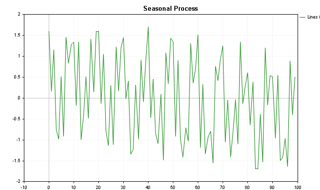
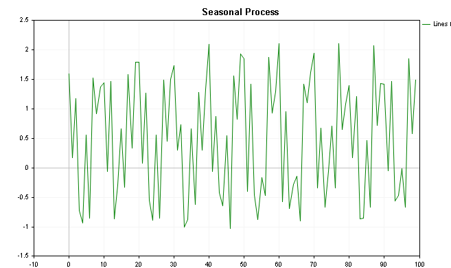
By putting the CSpectrum class to work we can visualize the power spectrum of this series as shown below. We can see that the power spectrum clearly shows a few prominent peaks.

CSpectrumAnalysis sp(true,inputs); 
       
   sp.Plot(PLOT_POWER_SPECTRUM);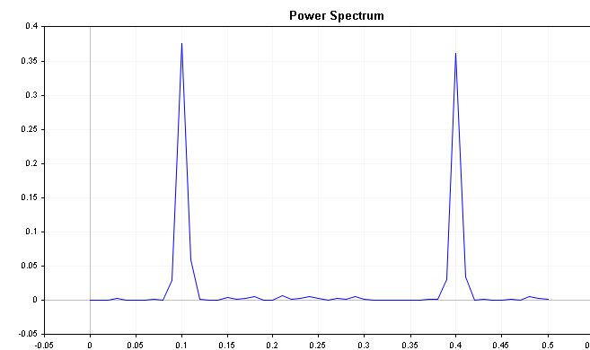 

The plot clearly shows that the series is strongly influenced by frequency components at 0.2 and 0.4 respectively.

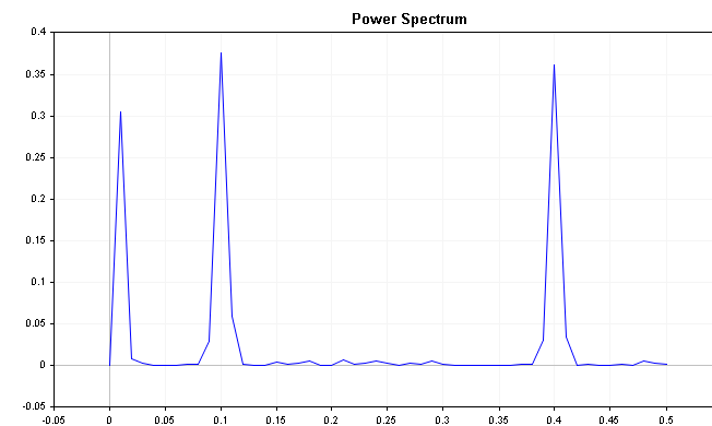
The spectrum of the series with a slight downward trend shows an initial peak along with the seasonal component. In such a situation it may be prudent to not only difference the series but to apply seasonal deferencing. It should be noted that the existence of such peaks is not always an indication of a trend/and or seasonality. The example shown has a fairly tame noise component where as  real world datasets such as financial series are plagued by distracting noise. Seasonality in a series usually shows up as an obvious peak in the power spectrum plot.

Determining the order of an autoregressive (AR) model

Autoregressive models are commonly used in time series analysis to predict future values of a series based on its past values. The order of the AR model determines how many past values are used to predict the next value. One method to determine the appropriate order for an AR model is to examine the power spectrum of the time series.

Typically, the power spectrum will decay as the frequency increases. For example, a time series that is defined by a  short-term positive autoregressive term  will have most of its spectral energy concentrated at low frequencies, while a series with short-term negative autoregressive term will shift its spectral energy to high frequencies.
Lets see what this looks like in practice by using another deterministic series defined by either a positive or negative autoregressive component. The code for generating the series is shown below.

double inputs[300];
   ArrayInitialize(inputs,0);

   MathSrand(2023);

   for(int i=1; i<ArraySize(inputs); i++)
     {
      inputs[i]= 0.0;
      
          switch(Coeff_Mult)
             {
              case positive:
               inputs[i]+= 0.9*inputs[i-1];
               break;
              case negative:
               inputs[i]+= -1*0.9*inputs[i-1];
               break;   
             }
             
      inputs[i]+=(double)rand() / double(SHORT_MAX);
     }

When the series is defined by  positive autoregression the power spectrum shows  most of the energy is concentrated at the low frequencies with the power at higher frequencies decreasing as one moves across the extent of the values.

Compare this with the plot of the autoregressive series with a negative term, we see that the power increases when sampling higher frequencies. Again this an easy example but it demonstrates important characteristics that can be applied when building autoregressive models.

Examining the spectrum of an error distribution to assess the performance of a prediction model

Finally, we can use the power spectrum of the error distribution of a prediction model to evaluate how well it models a process. To do this, we first, fit a prediction model to the time series data and calculate the residuals or errors (the difference between predicted and actual values).

Next,we examine the power spectrum of the error distribution. A good prediction model will have residuals that are white noise, which means that the power spectrum of the error distribution should be relatively flat across all frequencies. Prominent peaks in the power spectrum at any frequency suggest that the prediction model is not capturing all of the information in the time series data and further tuning may be necessary. The problem is that in reality the power spectrum of white noise is not usually flat as is expected. Just look at the spectrum of a white noise series generated from the code below.

int num_samples = 500;
   double inputs[];
   MathSrand(2023);
   ArrayResize(inputs,num_samples);
   
   for (int i = 0; i < num_samples; i++) 
    {
        inputs[i] = ((double)rand() / SHORT_MAX) * 32767 - 32767/2;
    }

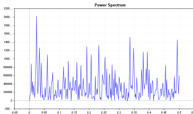
To get a clearer picture of the frequency components we can use the cumulative power spectrum .

Theorectically if a time series is white noise, all the spectral terms would be equal, so the cumulative power spectrum plot is expected to be straight. In particular, the fraction of the total power accounted for up through each individual term should be equal to the fraction of the total number of terms cummulated. Mathematically, it means that the cumulative power of white noise has a deterministic expectation. The equation that defines the cumulative power for each sampled frequency band is shown below.

 
If the power spectrum shows a high concentration of energy in either low or high frequencies, we will see deviations from the theoretical waveform of white noise. Using this fact we can compute the deviation between the observed and theoretical cumulative spectra, which yields the cumulative spectrum deviation.

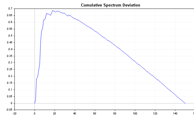
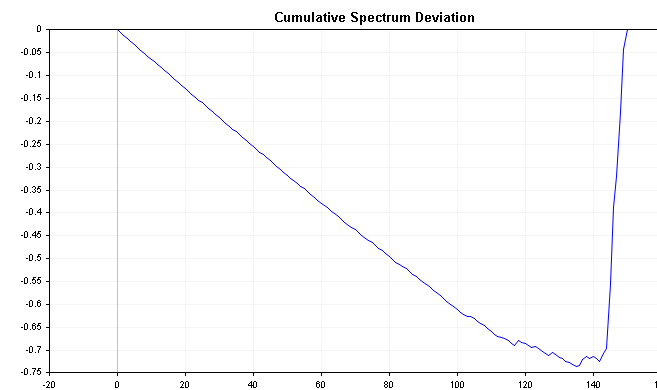
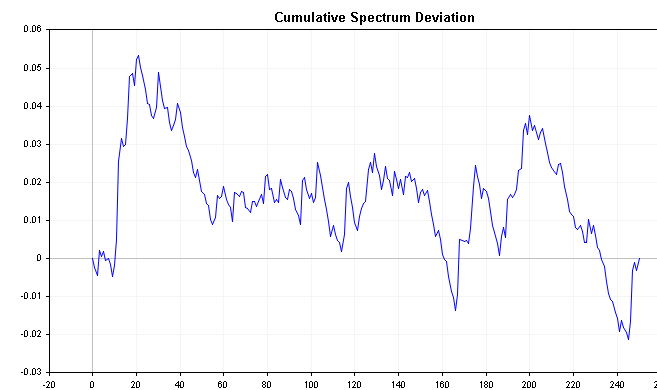
This series can reveal important information about the time series. For example, if the spectral energy is shifted to the left, the deviation will start off near zero and slowly increase until it converges much later. Conversely, if the spectral energy is shifted to the right, the deviation will immediately plunge to negative numbers and then slowly work its way back up to zero over time. White noise will produce deviation values that vary a lot less, relative to zero.

The plots below show the cumulative spectrum deviation of positive and negative AR(1) processes defined previously. Compare these with the cumulative spectrum plot of white noise , take note of the clearer distinctions.

 

It is known that the distribution of the maximum absolute value of all deviations follows the Komogoro Smirnov distribution. Applying the formula below we can test directly the hypothesis that the times series is white noise. This formula calculates the D statistic of a series.

q defines the degrees of freedom, if the dft is applied to a real time series , q =n/2-1. If a welch data window is applied before the dft, q must be multiplied by 0.72, to compensate for the loss of information brought on by windowing. Alpha is the significance level usually in percent. To test the white-noise hypothesis, get the maximum difference or deviation and compare it to the D statistic.

In the CSpectrum class the we can get the maximum difference determined by the cumulative spectrum deviation calculations by calling the CumulativeSpectrumDeviation() method.

Conclusion

The focus of this article has been on the dft for estimating the power spectrum of a time series, as it is well-known. However, there is an alternative method called the maximum entropy (ME) method that can sometimes outperform the dft. The ME spectrum has the ability to zoom in on very narrow features while smoothing areas with low spectral energy, resulting in a comprehensive display. However, the ME method has a tendency to find high spectral energy spikes even when they do not exist, making it unsuitable to be used alone. Hence, the dft spectrum should always be analyzed alongside it, serving as a second opinion, if you will.

In conclusion, analyzing the power spectrum of a time series data can provide valuable insights into various aspects of time series analysis, such as determining the order of an AR model, ascertaining the need for seasonal differencing as a preprocessing step, and examining the performance of prediction models.

File Name	Description
mql5files\include\Spectrum.mqh	Contains the definition of the CSpectrum class
mql5files\scripts\OrderOneARProcess.mql5	this script generates an autoregressive time series and applies the CSpectrum class
mql5files\scripts\SeasonalProcess.mql5	this script generates a time series  depicted by seasonality and applies the CSpectrum class
mql5files\scripts\WhiteNoise.mql5	this script generates a time series that is complete white noise and applies the CSpectrum class