Implementing an ARIMA training algorithm in MQL5

Introduction

Most forex and crypto traders that look to exploit short term movements are plagued by the lack of fundamental information that could aid their endeavours. This is where standard time series techniques could help . George Box and Gwilym Jenkins developed what is arguably the most revered method of time series prediction. Although a number of advances have come about that  improve on the original method, the underlying principles are still relevant today.

One of the derivatives of their methods is the Autoregressive Integrated Moving Average (ARIMA) which has become a popular method for time series forecasting. It is a class of models that captures temporal dependencies in a data series and provides a framework for modeling non-stationary time series. In this article, we will use Powells method of function minimization as a basis for the creation of an ARIMA training algorithm using the mql5 programming language.

Over view of ARIMA

Box and Jenkins stated that most time series could be modeled by one or both of two frameworks. One is Autoregressive (AR) which means that a value of a series can be explained in relation to its previous values along with a constant offset and a small difference, usually refered to as innovation or noise. Please note that in this text we will refer to the noise or error component as innovation. The innovation accounts for the random variation that cannot be explained.

The second framework underlying the ARIMA model is the Moving Average (MA).This model states that a value of a series is the proportional sum of a specific number of previous innovation terms , the current innovation and again, a constant offset. There are numerous other statistical conditions that define these models but we will not delve into the details. There are many resources available online that provide more information.We are more interested in their application.

We are not limited to pure MA and AR models only, we can combine them to produce mixed models called Autoregressive Moving Average models (ARMA). In an ARMA model we specify a finite number of lagged series and  noise terms in addition to a constant offset and a current innovation term.

One of the fundamental requirements that affects the application of all these frameworks is that the series being modeled needs to be stationary. Depending on how strict a definition of stationarity you are comfortable with, the models described so far are technically not appropriate for application with financial time series. This is where ARIMA comes in. Mathematical integration is the reverse of differentiation. When a non-stationary time series is differenced once or more times the resulting series usually has better stationarity. By first differencing a series it becomes possible to apply these models on the resulting series.The I in ARIMA refers to the requirement to reverse  (Integrate ) the differencing  applied in order to return the modeled series to its original domain

Autoregressive model notation

There is a standard notation that governs the description of a model. The number of AR terms (not including the constant term) is usually called p. The MA terms are denoted as q and d describes the number of times the original series has been differenced. Using these terms an ARIMA model is specified as ARIMA(p,d,q). Pure processes can be depicted as MA(q) and AR(p). Mixed models without differencing are written as ARMA(p,q). This notation assumes that the the terms are contiguous. For example ARMA(4,2) means the series can be described by 4 consecutive AR terms and  two previous consecutive innovation terms. Using ARIMA we able to depict pure processes by specifying either p,q or d as zero. An ARIMA(1,0,0) for example reduces to a pure AR(1) model.

Most autoregressive models specify that the respective terms are contiguous , from a lag of 1 to lag p and lag q for AR and MA terms respectively. The algorithm that will be demonstrated  will allow for the specification of non contiguous lags for either MA and/or AR terms. Another flexibility the algorithm will introduce is the ability to specify models with or without a constant offset.

For example it will be possible to build models defined by the function below:
                                 

                                                        y(t) = AR1* y(t-4) + AR2*y(t-6) + E(t)         (1)

The function above describes a pure AR(2) process without a constant offset  with the current value defined by the series values 4 and 6 previous time slots ago. The standard notation does not provide a way to specify such a model, but we need not be held back by such limitations.
 

Calculating model coefficients and the constant offset

A model can have p+q coefficients which must be calculated. To do so we use the specification of the model to make predictions of known series values then compare the predicted values against the known values and compute the sum of square errors . The optimal coefficients  will be those that produce the least sum of square errors.

Care must be take  when making predictions because of the limitations imposed by the unavailability of data that extends to infinity. If the model specification has any AR terms we can only start making predictions  after the number of values that correspond  with the largest lag of all the AR terms.

Using the example  specified by (1) above, we would only be able to start making predictions from time slot 7. As any prior predictions would reference unknown values before the start of the series.

It should be noted that if (1) had any MA terms , at this point the model would be treated as being purely autoregressive since we have no innovation series yet. The series of innovation values will be built up as prections are made going forward. Going back to the example the first prediction  at seventh time slot will be calculated with artibitrary initial AR coefficients.

 The difference between  the calculated  prediction and the known value at the seventh time slot  will be the innovation  for that slot. If there are any MA terms specified they will be included in the calculation of a prediction as  and when  the corresponding  lagged values of innovation become known. Otherwise the MA terms are just set to zero. In the case of a pure MA model a similar procedure is followed except this time, if a constant offset should be included it is initialized as the mean of the series .

There is only one obvious limitation to the method just described . The known series  needs to contain a commensurate number of values with respect  to the order of the model being applied. The more terms and /or  the larger the lags of those terms the more values we need to effectivley fit the model. The training process is then rounded off by applying an appropriate global minimization algorithm to optimize the coefficients. The algorithm we will use to minimize the prediction error is Powells method . The implementation details applied here are documented in the article Time Series Forecasting Using Exponential Smoothing.

The CArima class

The ARIMA training algorithm will be contained in the CArima class defined in Arima.mqh. The class  has two constructors each of which initialize an autoregressive model. The default constructor creates a pure AR(1) model with a constant offset.

CArima::CArima(void)
  {
   m_ar_order=1;
//---
   ArrayResize(m_arlags,m_ar_order);
   for(uint i=0; i<m_ar_order; i++)
      m_arlags[i]=i+1;
//---
   m_ma_order=m_diff_order=0;
   m_istrained=false;
   m_const=true;

   ArrayResize(m_model,m_ar_order+m_ma_order+m_const);
   ArrayInitialize(m_model,0);
  }

The parametized constructor allows more control in specifying a model. It takes four arguments listed below:

Parameter	Parameter Type	Parameter Description
p	unsigned integer	this specifies the number of AR terms for the model
d	unsigned integer	specifies the degree of differencing to be applied to a series being modeled
q	unsigned integer	indicates the number of  MA terms the model should contain
use_const_term	bool	sets the use of a constant offset in a model

CArima::CArima(const uint p,const uint d,const uint q,bool use_const_term=true)
  {
   m_ar_order=m_ma_order=m_diff_order=0;

   if(d)
      m_diff_order=d;
   if(p)
     {
      m_ar_order=p;
      ArrayResize(m_arlags,p);
      for(uint i=0; i<m_ar_order; i++)
         m_arlags[i]=i+1;
     }
   if(q)
     {
      m_ma_order=q;
      ArrayResize(m_malags,q);
      for(uint i=0; i<m_ma_order; i++)
         m_malags[i]=i+1;
     }


   m_istrained=false;
   m_const=use_const_term;

   ArrayResize(m_model,m_ar_order+m_ma_order+m_const);
   ArrayInitialize(m_model,0);
  }

In addition to the two constructors provided, a model can also be specified by using one of the over loaded  Fit() methods. Both methods  takes as their first  argument the data series to be modeled. One Fit() method has only one argument whilst a second requires four more arguments, all of which are identical to those already documented in the table above.

bool CArima::Fit(double &input_series[])
  {

   uint input_size=ArraySize(input_series);

   uint in = m_ar_order+ (m_ma_order*2);

   if(input_size<=0 || input_size<in)
      return false;

   if(m_diff_order)
      difference(m_diff_order,input_series,m_differenced,m_leads);
   else
      ArrayCopy(m_differenced,input_series);

   ArrayResize(m_innovation,ArraySize(m_differenced));

   double parameters[];
   ArrayResize(parameters,(m_const)?m_ar_order+m_ma_order+1:m_ar_order+m_ma_order);
   ArrayInitialize(parameters,0.0);

   int iterations = Optimize(parameters);

   if(iterations>0)
      m_istrained=true;
   else
      return false;

   m_sse=PowellsMethod::GetFret();

   ArrayCopy(m_model,parameters);

   return true;

  }

Using the method with more parameters overwrites any model that was previously specified and also assumes the lags of the terms are adjacent to one another. Both assume the data series specified as the first parameter is not differenced. So differencing will be applied if specified by the model parameters. The methods both return a boolean value denoting success or failure of the model training process.

bool CArima::Fit(double&input_series[],const uint p,const uint d,const uint q,bool use_const_term=true)
  {
   m_ar_order=m_ma_order=m_diff_order=0;

   if(d)
      m_diff_order=d;
   if(p)
     {
      m_ar_order=p;
      ArrayResize(m_arlags,p);
      for(uint i=0; i<m_ar_order; i++)
         m_arlags[i]=i+1;
     }
   if(q)
     {
      m_ma_order=q;
      ArrayResize(m_malags,q);
      for(uint i=0; i<m_ma_order; i++)
         m_malags[i]=i+1;
     }

   m_istrained=false;
   m_const=use_const_term;

   ZeroMemory(m_innovation);
   ZeroMemory(m_model);
   ZeroMemory(m_differenced);

   ArrayResize(m_model,m_ar_order+m_ma_order+m_const);
   ArrayInitialize(m_model,0);

   return Fit(input_series);

  }

With regards to setting the lags for the AR and MA terms, the class provides the methods SetARLags() and SetMALags() respectively. Both work similarly by taking a single array argument whose elements should be the corresponding lags for a model already specified by either of the constructors. The size of the array should match the corresponding order of AR or MA terms. The elements in the array can contain any value larger than or equal to one.  Let's look at an example of specifying a model with non adjacent  AR and MA lags.

The model we wish to build is specified by the function below:
         

                                        y(t) = AR1*y(t-2) + AR2*y(t-5) + MA1*E(t-1) + MA2*E(t-3) + E(t)                 (2)

This models is defined by an ARMA(2,2) process using AR lags of 2 and 5 . and MA lags of 1 and 3.
The code below shows how such a model can be specified.

CArima arima(2,0,2);

uint alags [2]= {2,5};
uint mlags [2]= {1,3};

if(arima.SetARLags(alags) && arima.SetMALags(mlags))
   Print(arima.Summary());

Upon successfully fitting a model to a data series by using one of the Fit() methods, the optimal coefficients and the constant offset can be retrieved by calling the GetModelParameters() method. It requires an array argument to which all the optimized parameters of the model will be written. The constant offset will be first followed by the AR terms and the MA terms will always be listed last.

class CArima:public PowellsMethod
  {
private:
   bool              m_const,m_istrained;
   uint              m_diff_order,m_ar_order,m_ma_order;
   uint              m_arlags[],m_malags[];
   double            m_model[],m_sse;
   double            m_differenced[],m_innovation[],m_leads[];

   void              difference(const uint difference_degree, double &data[], double &differenced[], double &leads[]);
   void              integrate(double &differenced[], double &leads[], double &integrated[]);
   virtual double    func(const double &p[]);


public :
                     CArima(void);
                     CArima(const uint p,const uint d, const uint q,bool use_const_term=true);
                    ~CArima(void);

   uint              GetMaxArLag(void)    { if(m_ar_order) return m_arlags[ArrayMaximum(m_arlags)]; else return 0;}
   uint              GetMinArLag(void)    { if(m_ar_order) return m_arlags[ArrayMinimum(m_arlags)]; else return 0;}
   uint              GetMaxMaLag(void)    { if(m_ma_order) return m_malags[ArrayMaximum(m_malags)]; else return 0;}
   uint              GetMinMaLag(void)    { if(m_ma_order) return m_malags[ArrayMinimum(m_malags)]; else return 0;}
   uint              GetArOrder(void)     { return m_ar_order;  }
   uint              GetMaOrder(void)     { return m_ma_order;  }
   uint              GetDiffOrder(void)   { return m_diff_order;}
   bool              IsTrained(void)      { return m_istrained; }
   double            GetSSE(void)         { return m_sse;      }
   uint              GetArLagAt(const uint shift);
   uint              GetMaLagAt(const uint shift);


   bool              SetARLags(uint &ar_lags[]);
   bool              SetMALags(uint &ma_lags[]);
   bool              Fit(double &input_series[]);
   bool              Fit(double &input_series[],const uint p,const uint d, const uint q,bool use_const_term=true);
   string            Summary(void);
   void              GetModelParameters(double &out_array[]) { ArrayCopy(out_array,m_model);      }
   void              GetModelInnovation(double &out_array[]) { ArrayCopy(out_array,m_innovation); }

  };

GetModelInnovation () writes to its single array argument the error values that calculated with the optimized coefficients after  fitting a model. Whilst the Summary () function returns a string description that details the full model.GetArOrder(), GetMaOrder() and GetDiffOrder() return the number of AR terms, MA terms and the degree of differening respectively for a model.

GetArLagAt() and GetMaLagAt() each take an unsigned integer argument that corresponds with the ordinal position of an AR or MA term. The zero shift references the first term. GetSSE() returns the sum of square errors for a trainned model. IsTrained() returns true or false depending on whether a specified model has been trainned or not.

Since CArima inherits from PowellsMethod, various parameters of Powell's algorithm can be adjusted. More details about PowellsMethod can be found here.

Using the CArima class

The code of the script below demonstrates how a model can be constructed and its parameters estimated for a deterministic series. In the demonstration presented in the script, a deterministic series will generated with the option to specify the constant offset value and the addition of a random componet which will mimic noise.

The script includes  Arima.mqh and fills the input array  with a series constructed from a deterministic and random component.

#include<Arima.mqh>

input bool Add_Noise=false;
input double Const_Offset=0.625;

We declare the a CArima object specifying a pure AR(2) model. The Fit() method with the input array is called and the results of training are displayed with the help of the Summary() function. Output of the script shown below.

double inputs[300];
   ArrayInitialize(inputs,0);

   int error_code;

   for(int i=2; i<ArraySize(inputs); i++)
     {
      inputs[i]= Const_Offset;
      inputs[i]+= 0.5*inputs[i-1] - 0.3*inputs[i-2];
      inputs[i]+=(Add_Noise)?MathRandomNormal(0,1,error_code):0;
     }

   CArima arima(2,0,0,Const_Offset!=0);

   if(arima.Fit(inputs))
      Print(arima.Summary());

The script is run twice with and without the noise component. In the first run we see that the algorithm was able to estimate the exact coefficients of the series. In second run, with added noise the algorithm did a fair job of reproducing the true constant offset and coefficients that defined our series.

The example demonstrated is obviously not representative of the type of analysis we will encounter in the real world. The noise added to the series was moderate relative to that encounted in financial time series.

Designing ARIMA models

So far we have looked at the implementation of an autoregressive training algorithm without indicating how to derive or choose the appropriate order for a model. Training a model is probably the easy part, in constrast to determining a good model.

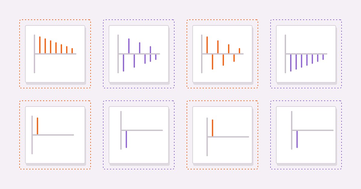
Two useful tools to derive a suitable model is to calculate the autocorrelation and partial autocorrelation of a series under study. As a guide to help readers in interpreting autocorrelation and partial autocorrelation plots we will consider four hypothetical series.
                                                                  y(t) = AR1* y(t-1) +  E(t)           (3) 

                 
                                                                  y(t) = E(t) - AR1 * y(t-1)            (4) 

            
                                                                  y(t) = MA1 * E(t-1) +  E(t)          (5) 

                
                                                                   y(t) = E(t) - MA1 * E(t-1)           (6) 

    
(3) and (4) are pure AR(1) processes with positive and negative coefficients respectively. (5) and (6) are pure MA(1) processes with positive and negative coefficients respectively.  

The figures above are the autocorrelations of (3) and (4)  respectively. In both plots the correlation values become smaller as the lag increases. This makes sense since the effect of a previous value on the current diminishes as one goes further up the series.

The next figures show the plots of partial autocorrelations of the same pair of series. We see that the correlation values cut off after the first lag. These observations provide the basis for a general rule about AR models. In general if partial autocorrelations cut off beyond a certain lag and the autocorrelations simultaneously begin to decay beyond the same lag  then the series can be modeled by a pure AR model up to the observed cut off lag on the partial autocorrelation plot.

 Examing the autocorrelation plots for the MA series we notice that the plots are  identical to the partial autocorrelations of the AR(1) .

In general if all autocorrelations beyond  a certain peak or trough are zero and the partial autocorrelations become ever smaller as more lags are sampled then the series can be defined by a MA term at the observed cutt off lag on the autocorrelation plot.

 
Other ways to determine the p and q parameters of a model include:

• Information Criteria: There are several information criteria, such as Akaike Information Criterion (AIC) and Bayesian Information Criterion (BIC), that can be used to compare different ARIMA models and select the best one.

• Grid Search: This involves fitting different ARIMA models with different orders on the same dataset and comparing their performance. The order that yields the best results is chosen as the optimal ARIMA order.

• Time Series Cross-Validation: This involves splitting your time series data into training and testing sets, fitting different ARIMA models on the training set, and evaluating their performance on the testing set. The ARIMA order that yields the best test error is chosen as the optimal order.

It's important to note that there is no one-size-fits-all approach to selecting the ARIMA order, and it may require some trial and error and domain knowledge to determine the best order for your specific time series.

Conclusion

We demonstrated the CArima class that encapsulates an autoregressive training algorithm using Powells method of function minimization. The code for the full class is given in the zip file attached below along with a script demonstrating its use.

File	Description
Arima.mqh	include file with definition of theCArima class
PowellsMethod.mqh	include file with definition of PowellsMethod class
TestArima	script that demonstrates the use of the CArima class to analyze a partially deterministic series.