数据科学与机器学习（第 03 部分）：矩阵回归

MetaTrader 5 — 示例 | 22 八月 2022, 07:47

1 076

Omega J Msigwa

经过长时间的反复试验，多元动态回归的谜题终于破解了...继续阅读。

如果您关注过前两篇文章，您会注意到我曾遇到的一个大难题，即是编程模型可以处理更多的自变量，我的意思是动态处理更多的输入，因为当涉及到创建策略时，我们需要处理数百个数据，所以我们希望确保我们的模型能够满足这一需求。

矩阵

对于那些跳过数学类的人，矩阵是一个矩形数组或数字表格或其它数学对象，按行和列排列，用于表示数学对象或此类对象的属性。

例如:

矩阵示例图像

房间里有一头大象。

我们读取矩阵的方式是行x列。上述矩阵是一个 2x3 矩阵，表示 2行，3列。

毋庸置疑，矩阵在现代计算机处理信息，和计算大数据的过程中起着巨大的作用，它们能够实现这一点的主要原因是矩阵中的数据以数组形式存储，且计算机可以轻易地读取和处理。我们看看它们在机器学习中的应用。

线性回归

矩阵允许线性代数形式的计算。因此，矩阵的研究是线性代数的重要组成部分，如此我们就可以用矩阵来建立线性回归模型。

正如我们所知，直线的方程是

标量形式方程的线性模型

其中，∈ 是误差项，Bo 和 Bi 分别是系数 y-截距，和斜率系数。

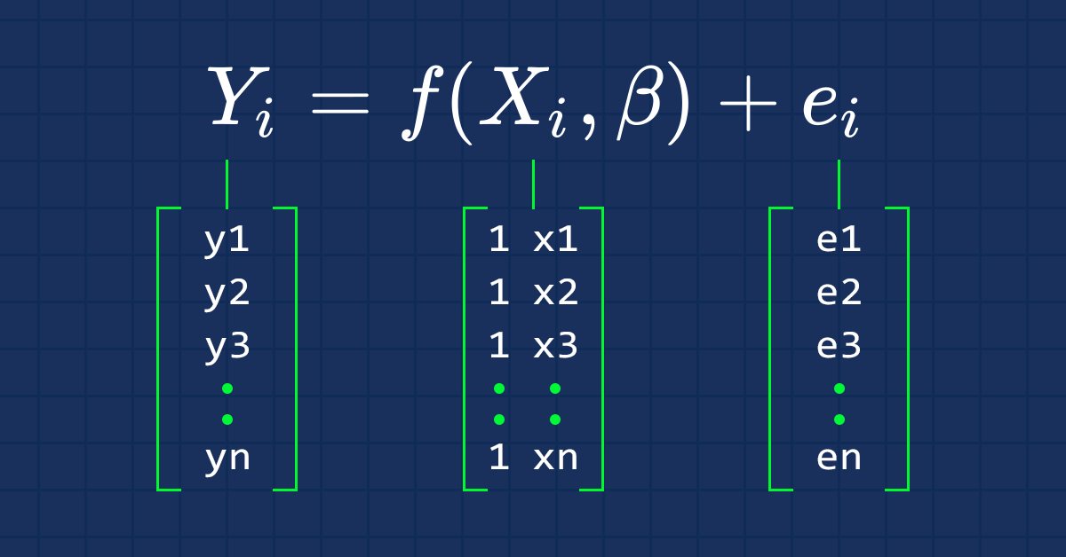
从现在起，我们对本系列文章感兴趣的是方程的向量形式。这就是

这是矩阵形式的简单线性回归公式。

对于简单的线性模型（和其它回归模型）我们感兴趣的通常是求斜率系数/普通最小二乘估计值。

向量 Beta 是包含 β 的向量。

Bo 和 B1，如来自等式的解释

线性回归方程的标量形式

我们感兴趣的是寻找系数，因为它们在建立模型时非常重要。

向量形式模型的评估公式为：

这是所有书呆子都要记住的一个非常重要的公式。我们将很快探讨如何找到公式中的元素。

xTx 的乘积将得出对称矩阵，因为 xT 中的列数与 x 中的行数相同，我们将在后面的操作中看到这一点。

如前所述，x 也引用为设计矩阵，以下是其矩阵的外观。

设计矩阵

正如您所看到的，我们在矩阵数组每一行的最开头第一列上，全部填充值 1，一直到矩阵的末行。这是为矩阵回归准备数据的第一步。当我们进一步计算时，您将看到这样做的好处。

我们在函数库的 Init() 函数中处理这个过程。

void CSimpleMatLinearRegression::Init(double &x[],double &y[], bool debugmode=true)
 {
    ArrayResize(Betas,2); //since it is simple linear Regression we only have two variables x and y
        
    if (ArraySize(x) != ArraySize(y))
      Alert("There is variance in the number of independent variables and dependent variables \n Calculations may fall short");
      
    m_rowsize = ArraySize(x);
    
    ArrayResize(m_xvalues,m_rowsize+m_rowsize); //add one row size space for the filled values 
    ArrayFill(m_xvalues,0,m_rowsize,1); //fill the first row with one(s) here is where the operation is performed
    
    ArrayCopy(m_xvalues,x,m_rowsize,0,WHOLE_ARRAY); //add x values to the array starting where the filled values ended
    ArrayCopy(m_yvalues,y);
    
    m_debug=debugmode;
 }

至此刻为止，当我们打印设计矩阵值时，这里是我们的输出，正如您可以看到的那样，一行中的填充值结束于 x 值开始的位置。

[ 0] 1.0 1.0 1.0 1.0 1.0 1.0 1.0 1.0 1.0 1.0 1.0 1.0 1.0 1.0 1.0 1.0 1.0 1.0 1.0 1.0 1.0

[ 21] 1.0 1.0 1.0 1.0 1.0 1.0 1.0 1.0 1.0 1.0 1.0 1.0 1.0 1.0 1.0 1.0 1.0 1.0 1.0 1.0 1.0

........

[ 693] 1.0 1.0 1.0 1.0 1.0 1.0 1.0 1.0 1.0 1.0 1.0 1.0 1.0 1.0 1.0 1.0 1.0 1.0 1.0 1.0 1.0

[ 714] 1.0 1.0 1.0 1.0 1.0 1.0 1.0 1.0 1.0 1.0 1.0 1.0 1.0 1.0 1.0 1.0 1.0 1.0 1.0 1.0 1.0

[ 735] 1.0 1.0 1.0 1.0 1.0 1.0 1.0 1.0 1.0 4173.8 4179.2 4182.7 4185.8 4180.8 4174.6 4174.9 4170.8 4182.2 4208.4 4247.1 4217.4

[ 756] 4225.9 4211.2 4244.1 4249.0 4228.3 4230.6 4235.9 4227.0 4225.0 4219.7 4216.2 4225.9 4229.9 4232.8 4226.4 4206.9 4204.6 4234.7 4240.7 4243.4 4247.7

........

[1449] 4436.4 4442.2 4439.5 4442.5 4436.2 4423.6 4416.8 4419.6 4427.0 4431.7 4372.7 4374.6 4357.9 4381.6 4345.8 4296.8 4321.0 4284.6 4310.9 4318.1 4328.0

[1470] 4334.0 4352.3 4350.6 4354.0 4340.1 4347.5 4361.3 4345.9 4346.5 4342.8 4351.7 4326.0 4323.2 4332.7 4352.5 4401.9 4405.2 4415.8

xT 或 x 转置是矩阵中的过程，通过该过程，我们将行与列的数据对换。

这意味着如果我们将这两个矩阵相乘

我们将跳过转置矩阵的过程，因为我们收集数据的方式本就是转置形式，尽管另一方面我们必须取消 x 值的转置，以便我们可以将它们与已经转置过的 x 矩阵相乘。

只是大喊一声，矩阵 nx2 并未转置，数组如下所示 [1 x1 1 x2 1 ... 1 xn]。我们来看一下这个动作。

X 矩阵取消转置

我们从 csv 文件中获得的转置矩阵在打印出来时如下所示：

转置矩阵

[

[ 0] 1 1 1 1 1 1 1 1 1 1 1 1 1 1 1 1 1 1 1 1 1 1 1 1 1 1 1 1 1 1 1 1 1 1 1 1 1 1 1 1 1 1 1 1 1 1 1 1 1 1

...

[ 0] 4174 4179 4183 4186 4181 4175 4175 4171 4182 4208 4247 4217 4226 4211 4244 4249 4228 4231 4236 4227 4225 4220 4216 4226

...

[720] 4297 4321 4285 4311 4318 4328 4334 4352 4351 4354 4340 4348 4361 4346 4346 4343 4352 4326 4323 4333 4352 4402 4405 4416

]

取消转置的过程是这样的，我们只需要将行与列数据互换，这与转置矩阵的过程相同。

    int tr_rows = m_rowsize,
        tr_cols = 1+1; //since we have one independent variable we add one for the space created by those values of one
        
    
    MatrixUnTranspose(m_xvalues,tr_cols,tr_rows);

    Print("UnTransposed Matrix");
    MatrixPrint(m_xvalues,tr_cols,tr_rows);

事情在此变得棘手。

我们将转置矩阵中的列放在一个应该是行的地方，而行则需要放于列的地方，运行此代码片段时的输出将是：

        UnTransposed Matrix
        [ 
            1  4248
            1  4201
            1  4352
            1  4402
...
...
            1  4405
            1  4416
        ]

xT 是一个 2xn 矩阵，x 是一个 nx2。得到的矩阵将是一个 2x2 矩阵。

那么，我们来看看它们相乘后的乘积是什么样子。

注意：若要令矩阵相乘变为可能，第一个矩阵中的列数必须等于第二个矩阵中的行数。

请参见此链接上的矩阵乘法规则 https://zh.wikipedia.org/wiki/Matrix_multiplication。

在该矩阵中执行乘法的方式是：

行 1 乘以列 1
行 1 乘以列 2
行 2 乘以列 1
行 2 乘以列 2

从我们的矩阵行 1 乘以列 1，输出将是迭代行 1 的每个元素，与列 1 对应索引位置的元素相乘，并把乘积累加求和，由于行 1 都是数值 1，列 1 也是数值 1，故这与在迭代中每次逐一递增值没有什么区别。

注意：

如果您想知道数据集合中的观测数量，可以依赖于在 xTx 输出中第一行第一列数量。

行 1 乘以列 2。由于行 1 包含值 1，当我们计算行 1（即值 1）与列 2（即值 x）的乘积累加时，输出将是 x 项的总和，因为乘以 1 没有影响。

行 2 乘以列 1。输出将是 x 的总和，因为来自 行 2 中的值 1 与 列 1 中的值 x 相乘时不起作用。

最后一部分是 x 值的平方和。

因为它是 row2 的包含值 x 与 colum2 的包含值 x 乘积后之和

如您所见，在这种情况下，矩阵的输出是一个 2x2 矩阵。

我们看看这在现实世界中是如何工作的，利用来自线性回归中第一篇文章中的数据集合 https://www.mql5.com/zh/articles/10459。我们提取数据，并将其放入一个数组中，自变量为 x，而因变量为 y。

//inside MatrixRegTest.mq5 script

#include "MatrixRegression.mqh";
#include "LinearRegressionLib.mqh";
CSimpleMatLinearRegression matlr;
CSimpleLinearRegression lr; 
//+------------------------------------------------------------------+
//| Script program start function                                    |
//+------------------------------------------------------------------+
void OnStart()
  {
    //double x[] = {651,762,856,1063,1190,1298,1421,1440,1518}; //stands for sales
    //double y[] = {23,26,30,34,43,48,52,57,58}; //money spent on ads
//---
    double x[], y[];
    string file_name = "NASDAQ_DATA.csv", delimiter = ",";
    
    lr.GetDataToArray(x,file_name,delimiter,1);
    lr.GetDataToArray(y,file_name,delimiter,2);
    
}

于此，我已经导入了我们在第一篇文章中创建的 CsimpleLinearRegression 函数库。

CSimpleLinearRegression lr;

因为我们可能需要调用某些函数，例如提取数据放到数组。

我们来寻找 xTx

MatrixMultiply(xT,m_xvalues,xTx,tr_cols,tr_rows,tr_rows,tr_cols);
    
Print("xTx");
MatrixPrint(xTx,tr_cols,tr_cols,5); //remember?? the output of the matrix will be the row1 and col2 marked in red

如果您注意数组 xT[] 的话，您可能发现我们只是复制了 x 值，并将它们存储在这个 xT[]数组中，它只是为了澄清，正如我早前所说的，我们所用的从 csv 文件收集数据并存于数组方式，调用函数 GetDataToArray() 得到的数据已经过转置。

然后我们将数组 xT[] 乘以已转置的 m_xvalues[] ，m_xvalues 是在函数库中定义的全局数组，用于存储 x 值。这是我们的 MatrixMultiply() 函数的内部。

void CSimpleMatLinearRegression::MatrixMultiply(double &A[],double &B[],double &output_arr[],int row1,int col1,int row2,int col2)
 {
//---   
   double MultPl_Mat[]; //where the multiplications will be stored
   
   if (col1 != row2)
        Alert("Matrix Multiplication Error, \n The number of columns in the first matrix is not equal to the number of rows in second matrix");
 
   else 
    { 
        ArrayResize(MultPl_Mat,row1*col2);
        
        int mat1_index, mat2_index;
        
        if (col1==1)  //Multiplication for 1D Array
         {
            for (int i=0; i<row1; i++)
              for(int k=0; k<row1; k++)
                 {
                   int index = k + (i*row1);
                   MultPl_Mat[index] = A[i] * B[k];
                 }
           //Print("Matrix Multiplication output");
           //ArrayPrint(MultPl_Mat);
         }
        else 
         {
         //if the matrix has more than 2 dimensionals
         for (int i=0; i<row1; i++)
          for (int j=0; j<col2; j++)
            { 
               int index = j + (i*col2);
               MultPl_Mat[index] = 0;
               
               for (int k=0; k<col1; k++)
                 {
                     mat1_index = k + (i*row2);   //k + (i*row2)
                     mat2_index = j + (k*col2);   //j + (k*col2)
                     
                     //Print("index out ",index," index a ",mat1_index," index b ",mat2_index);
                     
                       MultPl_Mat[index] += A[mat1_index] * B[mat2_index];
                       DBL_MAX_MIN(MultPl_Mat[index]);
                 }
               //Print(index," ",MultPl_Mat[index]);
             }
           ArrayCopy(output_arr,MultPl_Mat);
           ArrayFree(MultPl_Mat);
       }
    }
 }

诚恳地讲，这种乘法看起来既混乱又丑陋，尤其是在这样的情况下

k + (i*row2); 
j + (k*col2);

已在使用。 放轻松，兄弟！这就是我操纵这些索引的方式，如此它们即可为我们提供特定行和列的索引。如果我可以使用二维数组，例如 Matrix[rows][columns] ，这就很容易理解，在这种情况下，这将是 Matrix[i][k]，但我选择不这样用，因为多维数组有局限性，所以我必须找到一种方法。我在文章末尾链接了一些简单的 c++代码，我认为这些代码可以帮助您理解我是如何做到这一点的，或者您可以阅读本博客来了解更多有关的信息 https://www.programiz.com/cpp-programming/examples/matrix-multiplication。

调用 MatrixPrint() 函数成功输出 xTx：

 Print("xTx");
 MatrixPrint(xTx,tr_cols,tr_cols,5);
xTx
[ 
    744.00000 3257845.70000
    3257845.70000 14275586746.32998

]

正如您所看到的，我们的 xTx 数组中的第一个元素含有数据集合中每个数据的观测值数量，这就是为什么在设计矩阵时，第一列填充一个初始值非常重要的原因。

现在让我们来求 xTx 的逆矩阵。.

xTx 的逆矩阵

为了找到 2x2 矩阵的逆矩阵，我们首先交换对角线的第一个和最后一个元素，然后在其它两个值上添加负号。

公式如下图所示：

求矩阵的行列式 det(xTx) = 第一对角线的乘积 - 第二对角线的乘积。

下面是我们如何在 mql5 代码中求逆的结果

void CSimpleMatLinearRegression::MatrixInverse(double &Matrix[],double &output_mat[]) 
{
// According to Matrix Rules the Inverse of a matrix can only be found when the 
// Matrix is Identical Starting from a 2x2 matrix so this is our starting point
   
   int matrix_size = ArraySize(Matrix);

   if (matrix_size > 4)
     Print("Matrix allowed using this method is a 2x2 matrix Only");
  
  if (matrix_size==4)
     {
       MatrixtypeSquare(matrix_size);
       //first step is we swap the first and the last value of the matrix
       //so far we know that the last value is equal to arraysize minus one
       int last_mat = matrix_size-1;
       
       ArrayCopy(output_mat,Matrix);
       
       // first diagonal
       output_mat[0] = Matrix[last_mat]; //swap first array with last one
       output_mat[last_mat] = Matrix[0]; //swap the last array with the first one
       double first_diagonal = output_mat[0]*output_mat[last_mat];
       
       // second diagonal  //adiing negative signs >>>
       output_mat[1] = - Matrix[1]; 
       output_mat[2] = - Matrix[2];
       double second_diagonal = output_mat[1]*output_mat[2]; 
       
       if (m_debug)
        {
          Print("Diagonal already Swapped Matrix");
          MatrixPrint(output_mat,2,2);
        }
        
       //formula for inverse is 1/det(xTx) * (xtx)-1
       //determinant equals the product of the first diagonal minus the product of the second diagonal
       
       double det =  first_diagonal-second_diagonal;
       
       if (m_debug)
       Print("determinant =",det);
       
       
       for (int i=0; i<matrix_size; i++)
          { output_mat[i] = output_mat[i]*(1/det); DBL_MAX_MIN(output_mat[i]); }
       
     }
 }

运行此代码模块的输出将是

	Diagonal already Swapped Matrix
	[ 
	 14275586746     -3257846
	 -3257846       744
	]
	determinant =7477934261.0234375

我们打印该矩阵的逆矩阵，看看它是什么样子

       Print("inverse xtx");
       MatrixPrint(inverse_xTx,2,2,_digits); //inverse of simple lr will always be a 2x2 matrix

输出肯定是

[

1.9090281 -0.0004357

-0.0004357 0.0000001

]

现在我们已有了 xTx 逆矩阵，我们继续。

求 xTy

在此，我们将 xT[] 与 y[] 值相乘

    double xTy[];
    MatrixMultiply(xT,m_yvalues,xTy,tr_cols,tr_rows,tr_rows,1); //1 at the end is because the y values matrix will always have one column which is it    

    Print("xTy");
    MatrixPrint(xTy,tr_rows,1,_digits); //remember again??? how we find the output of our matrix row1 x column2

输出肯定是

xTy

[

10550016.7000000 46241904488.2699585

]

参考公式

现在我们有了 xTx 逆矩阵 和 xTy，我们整理一下。

   MatrixMultiply(inverse_xTx,xTy,Betas,2,2,2,1); //inverse is a square 2x2 matrix while xty is a 2x1
    
   
   Print("coefficients");
   MatrixPrint(Betas,2,1,5); // for simple lr our betas matrix will be a 2x1

有关我们如何调用函数的更多详细信息。

此代码片段的输出将是

coefficients

[

-5524.40278 4.49996

]

B A M !!! 这与我们在本系列文章的第 01 部分中通过标量形式的模型获得的系数结果相同。

Betas 数组的第一个索引处的数字将始终是 Constant/ Y- Intercept。我们最初能够获得它的原因是因为我们在设计矩阵时，在第一列中填充了值 1，这再次验证了该过程的重要性。它为 y-截距留下空间，令其留在该列中。

现在，我们完成了简单的线性回归。我们看看多元回归会是什么样子。请密切关注，因为事情可能变得越发棘手、复杂数倍。

多元动态回归难题解决

基于矩阵构建模型的好处是，在构建模型时，很容易扩展模型，而无需对代码进行太多修改。关于多元回归，您会注意到的一个重要变化就是矩阵如何求逆，因为这是我花了很长时间试图解决的最困难的部分，我会在后面的章节中详细介绍，但现在，我们在多元矩阵回归函数库中编写可能需要的代码。

我们可以只用一个函数库来处理简单和多元回归，简单地输入函数参数即可，但我决定创建另一个文件，如此来澄清一些事情，因为只要您理解了我刚才解释的简单线性回归部分中执行的计算，那该过程将几乎相同。

首先，我们针对函数库中可能需要的基本内容进行编码。

class CMultipleMatLinearReg
  {
      private:             
      
                           int     m_handle;
                           string  m_filename;
                           string  DataColumnNames[];    //store the column names from csv file
                           int     rows_total;
                           int     x_columns_chosen;     //Number of x columns chosen
                           
                           bool    m_debug;
                           double  m_yvalues[];     //y values or dependent values matrix
                           double  m_allxvalues[];  //All x values design matrix
                           string  m_XColsArray[];  //store the x columns chosen on the Init 
                           string  m_delimiter;
                           
                           double  Betas[]; //Array for storing the coefficients 
  
      protected:
                           
                           bool    fileopen(); 
                           void    GetAllDataToArray(double& array[]);
                           void    GetColumnDatatoArray(int from_column_number, double &toArr[]);
      public:
      
                           CMultipleMatLinearReg(void);
                          ~CMultipleMatLinearReg(void);
                          
                           void Init(int y_column, string x_columns="", string filename = NULL, string delimiter = ",", bool debugmode=true);
  };

这就是 Init() 函数内部发生的情况

void CMultipleMatLinearReg::Init(int y_column,string x_columns="",string filename=NULL,string delimiter=",",bool debugmode=true)
 {
//--- pass some inputs to the global inputs since they are reusable

   m_filename = filename;
   m_debug = debugmode;
   m_delimiter = delimiter;
   
//---

   ushort separator = StringGetCharacter(m_delimiter,0);
   StringSplit(x_columns,separator,m_XColsArray);
   x_columns_chosen = ArraySize(m_XColsArray);
   ArrayResize(DataColumnNames,x_columns_chosen); 

//---

   if (m_debug) 
    {
      Print("Init, number of X columns chosen =",x_columns_chosen);
      ArrayPrint(m_XColsArray);
    }
    
//---
     
   GetAllDataToArray(m_allxvalues);
   GetColumnDatatoArray(y_column,m_yvalues);
   
   
// check for variance in the data set by dividing the rows total size by the number of x columns selected, there shouldn't be a reminder
   
   if (rows_total % x_columns_chosen != 0)
     Alert("There are variance(s) in your dataset columns sizes, This may Lead to Incorrect calculations");
   else
     {
      //--- Refill the first row of a design matrix with the values of 1   
       int single_rowsize = rows_total/x_columns_chosen;
       double Temp_x[]; //Temporary x array
       
       ArrayResize(Temp_x,single_rowsize);
       ArrayFill(Temp_x,0,single_rowsize,1);
       ArrayCopy(Temp_x,m_allxvalues,single_rowsize,0,WHOLE_ARRAY); //after filling the values of one fill the remaining space with values of x
      
       //Print("Temp x arr size =",ArraySize(Temp_x));
       ArrayCopy(m_allxvalues,Temp_x);
       ArrayFree(Temp_x); //we no longer need this array
       
       int tr_cols = x_columns_chosen+1,
           tr_rows = single_rowsize;
       
       ArrayCopy(xT,m_allxvalues);  //store the transposed values to their global array before we untranspose them
       MatrixUnTranspose(m_allxvalues,tr_cols,tr_rows); //we add one to leave the space for the values of one
       
       if (m_debug)
         {
           Print("Design matrix");
           MatrixPrint(m_allxvalues,tr_cols,tr_rows);
         } 
     }
 }

关于所做工作的更多细节

ushort separator = StringGetCharacter(m_delimiter,0);
StringSplit(x_columns,separator,m_XColsArray);
x_columns_chosen = ArraySize(m_XColsArray);
ArrayResize(DataColumnNames,x_columns_chosen);

此处，我们得到了在调用 TestScript 中的 Init 函数时所选的 x 列（自变量），然后我们将这些列存储到全局数组 m_XColsArray 当中，将列存储到数组中会有很多优点，因为我们很快将读取它们，如此我们就可以按照所有 x 值（自变量矩阵）/设计矩阵的数组的正确顺序存储它们。

我们还必须确保数据集合中所有行都是相同的，因为一旦某一行或某一列存在差异，那么所有计算都将失败。

if (rows_total % x_columns_chosen != 0)
   Alert("There are variances in your dataset columns sizes, This may Lead to Incorrect calculations");

然后，我们将所有 x 列数据转换为所有自变量的一个矩阵/设计矩阵/数组（您可以选择这些名称中的一个来称呼它们）。

GetAllDataToArray(m_allxvalues);

我们还打算将所有因变量存储到其矩阵当中。

GetColumnDatatoArray(y_column,m_yvalues);

这是设计矩阵准备好进行计算的关键步骤。如早前这里所述，在 x 值矩阵的第一列填充值 1。

  {
      //--- Refill the first row of a design matrix with the values of 1   
       int single_rowsize = rows_total/x_columns_chosen;
       double Temp_x[]; //Temporary x array
       
       ArrayResize(Temp_x,single_rowsize);
       ArrayFill(Temp_x,0,single_rowsize,1);
       ArrayCopy(Temp_x,m_allxvalues,single_rowsize,0,WHOLE_ARRAY); //after filling the values of one fill the remaining space with values of x
      
       //Print("Temp x arr size =",ArraySize(Temp_x));
       ArrayCopy(m_allxvalues,Temp_x);
       ArrayFree(Temp_x); //we no longer need this array
       
       int tr_cols = x_columns_chosen+1,
           tr_rows = single_rowsize;
       
       MatrixUnTranspose(m_allxvalues,tr_cols,tr_rows); //we add one to leave the space for the values of one
       
       if (m_debug)
         {
           Print("Design matrix");
           MatrixPrint(m_allxvalues,tr_cols,tr_rows);
         } 
     }

这一次，我们在初始化函数库时打印未转置的矩阵。

这就是我们针对 Init 函数上所需的一切，现在我们在 multipleMapTregTestScript.mq5 中调用它（链接在本文末尾）

#include "multipleMatLinearReg.mqh";
CMultipleMatLinearReg matreg;
//+------------------------------------------------------------------+
//| Script program start function                                    |
//+------------------------------------------------------------------+
void OnStart()
  {
//---
      string filename= "NASDAQ_DATA.csv";
      matreg.Init(2,"1,3,4",filename);
  }

脚本成功运行后的输出将是（这只是一个概貌）：

        Init, number of X columns chosen =3
        "1" "3" "4"
        All data Array Size 2232 consuming 52 bytes of memory
        Design matrix Array
        [ 
             1   4174  13387     35
             1   4179  13397     37
             1   4183  13407     38
             1   4186  13417     37
             ......
             ......
             1   4352  14225     47
             1   4402  14226     56
             1   4405  14224     56
             1   4416  14223     60
        ]

求解 xTx

就像我们在简单回归中所做的一样，这里的过程是相同的，我们从 csv 文件中获取 xT 值的原始数据，然后将其与未转置矩阵相乘。

    MatrixMultiply(xT,m_allxvalues,xTx,tr_cols,tr_rows,tr_rows,tr_cols);

打印 xTx 矩阵时的输出将为：

   xTx
        [ 
             744.00  3257845.70 10572577.80    36252.20
            3257845.70 14275586746.33 46332484402.07   159174265.78
            10572577.80  46332484402.07 150405691938.78    515152629.66
            36252.20 159174265.78 515152629.66   1910130.22
        ]

酷，它的工作一如预期。

xTx 求逆

这是多元回归中最重要的部分，您应该密切关注，因为我们即将深入数学部分，事情即将变得复杂数倍。

上一部分中当我们在求解 xTx 的逆矩阵时，我们找到了 2x2 矩阵的逆矩阵，但这次我们要求解 4x4 的逆矩阵，因为我们选择了 3 列作为自变量，当我们将一列的值相加时，我们将得到 4 列，这就会导致我们在尝试求逆时得到 4x4 矩阵。

我们不能再用之前求逆的方法了，这次真正的问题是为什么？

请参见求逆矩阵的行列式方法，当矩阵很大时我们以前所用的方法已经无效了，甚至您都不能用它求解 3x3 的逆矩阵。

不同的数学家在求解逆矩阵时发明了若干种方法，其中一种是经典的伴随方法。但经过我的研究，这些方法中大多数都难以编码，有时会令人困惑。如果您想了解更多关于这些方法的详细信息，以及它们如何编码，请查看这篇博文 - https://www.geertarien.com/blog/2017/05/15/different-methods-for-matrix-inversion/。

在所有方法中，我选择采用高斯-乔丹（Gauss-Jordan）消元法，因为我发现它是可靠的，易于编码，易于扩展，这里有一个很棒的视频https://www.youtube.com/watch?v=YcP_KOB6KpQ，它很好地解释了高斯·乔丹，我希望这能帮助您理解这个概念。

好的，我们来编写高斯·乔丹（Gauss-Jordan），如果您发现代码很难理解，我有一个 c++ 代码，与下面链接的代码相同，而且下面的链接指向我的 GitHub，这可能有助于您理解这些事情是如何完成的。

void CMultipleMatLinearReg::Gauss_JordanInverse(double &Matrix[],double &output_Mat[],int mat_order)
 {
 
    int rowsCols = mat_order;
    
//--- 
       Print("row cols ",rowsCols);
       if (mat_order <= 2) 
          Alert("To find the Inverse of a matrix Using this method, it order has to be greater that 2 ie more than 2x2 matrix");
       else
         {
           int size =  (int)MathPow(mat_order,2); //since the array has to be a square
              
// Create a multiplicative identity matrix 

               int start = 0; 
               double Identity_Mat[];
               ArrayResize(Identity_Mat,size);
               
               for (int i=0; i<size; i++) 
                 {
                     if (i==start)
                       {
                        Identity_Mat[i] = 1;
                        start += rowsCols+1;
                       }
                     else 
                        Identity_Mat[i] = 0;
                        
                 }
                 
               //Print("Multiplicative Indentity Matrix");
               //ArrayPrint(Identity_Mat);
               
//---
      
              double MatnIdent[]; //original matrix sided with identity matrix
              
              start = 0;
              for (int i=0; i<rowsCols; i++) //operation to append Identical matrix to an original one
                {
                   
                   ArrayCopy(MatnIdent,Matrix,ArraySize(MatnIdent),start,rowsCols); //add the identity matrix to the end 
                   ArrayCopy(MatnIdent,Identity_Mat,ArraySize(MatnIdent),start,rowsCols);
                  
                  start += rowsCols;
                }
              
//---
   
               int diagonal_index = 0, index =0; start = 0;
               double ratio = 0; 
               for (int i=0; i<rowsCols; i++)
                  {  
                     if (MatnIdent[diagonal_index] == 0)
                        Print("Mathematical Error, Diagonal has zero value");
                     
                     for (int j=0; j<rowsCols; j++)
                       if (i != j) //if we are not on the diagonal
                         {
                           /* i stands for rows while j for columns, In finding the ratio we keep the rows constant while 
                              incrementing the columns that are not on the diagonal on the above if statement this helps us to 
                              Access array value based on both rows and columns   */
                            
                            int i__i = i + (i*rowsCols*2);
                            
                            diagonal_index = i__i;
                                                        
                            int mat_ind = (i)+(j*rowsCols*2); //row number + (column number) AKA i__j 
                            ratio = MatnIdent[mat_ind] / MatnIdent[diagonal_index];
                            DBL_MAX_MIN(MatnIdent[mat_ind]); DBL_MAX_MIN(MatnIdent[diagonal_index]);
                            //printf("Numerator = %.4f denominator =%.4f  ratio =%.4f ",MatnIdent[mat_ind],MatnIdent[diagonal_index],ratio);
                            
                             for (int k=0; k<rowsCols*2; k++)
                                {
                                   int j_k, i_k; //first element for column second for row
                                   
                                    j_k = k + (j*(rowsCols*2));
                                    
                                    i_k = k + (i*(rowsCols*2));
                                    
                                     //Print("val =",MatnIdent[j_k]," val = ",MatnIdent[i_k]);
                                     
                                                                        //printf("\n jk val =%.4f, ratio = %.4f , ik val =%.4f ",MatnIdent[j_k], ratio, MatnIdent[i_k]);
                                                                        
                                     MatnIdent[j_k] = MatnIdent[j_k] - ratio*MatnIdent[i_k];
                                     DBL_MAX_MIN(MatnIdent[j_k]); DBL_MAX_MIN(ratio*MatnIdent[i_k]);                                    
                                }
                                
                         }
                  }
                  
// Row Operation to make Principal diagonal to 1
             
/*back to our MatrixandIdentical Matrix Array then we'll perform 
operations to make its principal diagonal to 1 */
     
             
             ArrayResize(output_Mat,size);
             
             int counter=0;
             for (int i=0; i<rowsCols; i++)
               for (int j=rowsCols; j<2*rowsCols; j++)
                 {
                   int i_j, i_i;
                    
                    i_j = j + (i*(rowsCols*2));
                    i_i = i + (i*(rowsCols*2));
                    
                    //Print("i_j ",i_j," val = ",MatnIdent[i_j]," i_i =",i_i," val =",MatnIdent[i_i]);  
                    
                    MatnIdent[i_j] = MatnIdent[i_j] / MatnIdent[i_i];   
                    //printf("%d Mathematical operation =%.4f",i_j, MatnIdent[i_j]); 

                    output_Mat[counter]= MatnIdent[i_j];  //store the Inverse of Matrix in the output Array
                    
                    counter++;
                 }
                            
         }
//---

 }

太好了，我们调用函数，并打印逆矩阵

    double inverse_xTx[];
    Gauss_JordanInverse(xTx,inverse_xTx,tr_cols);
    
    if (m_debug)
      {
         Print("xtx Inverse");
         MatrixPrint(inverse_xTx,tr_cols,tr_cols,7);
      }

输出肯定是这样的，

        xtx Inverse
        [ 
         3.8264763 -0.0024984  0.0004760  0.0072008
        -0.0024984  0.0000024 -0.0000005 -0.0000073
         0.0004760 -0.0000005  0.0000001  0.0000016
         0.0072008 -0.0000073  0.0000016  0.0000290
        ]

记住，为了求解逆矩阵，它必须是一个方阵，所以在函数参数上，我们的参数 mat_order 等于行数和列数。

求 xTy

现在，我们求解 x 转置和 Y 的矩阵乘积。它与我们在之前所做的过程相同。

double xTy[];
MatrixMultiply(xT,m_yvalues,xTy,tr_cols,tr_rows,tr_rows,1); //remember!! the value of 1 at the end is because we have only one dependent variable y

当打印输出时，如下所示

 xTy
        [ 
            10550016.70000  46241904488.26996 150084914994.69019    516408161.98000
        ]

酷，如预期的一个 1x4 矩阵。

参考公式。

现在我们有了求解系数所需的一切，我们来整理一下。

     MatrixMultiply(inverse_xTx,xTy,Betas,tr_cols,tr_cols,tr_cols,1);

输出将是（再次记住，系数/β 矩阵的第一个元素是常数，或者换句话说是 y-截距）：

        Coefficients Matrix
        [ 
        -3670.97167     2.75527     0.37952     8.06681
        ]

太棒了！现在我用 python 来证明我错了。

python 得到的多元矩阵回归结果

双倍 B A M ! ! ! 这次

现在，以 mql5 实现多个动态回归模型终于成为可能，现在我们看看它从哪里开始。

一切始于这里

  matreg.Init(2,"1,3,4",filename);

这个思路是要有一个字符串输入，它可以帮助我们输入无限数量的自变量，而且在 mql5 中，我们似乎无法像 python 等语言那样允许我们从 *args" 和 *kwargs" 输入里得到很多参数。如此，我们唯一的方法是利用字符串，然后找到一种方法来让我们能够操纵数组，只需单一数组即可让我们拥有所有的数据，然后我们可以再找到一种方式来操纵它们。有关更多信息，请参阅我的第一次失败尝试 https://www.mql5.com/zh/code/38894，我之所以这么说，是因为我相信有人可能会在这个或那个项目上迈入同样的道路，我在此只是在解释什么对我有效，什么对我无效。