Solving Gold Market Overfitting: A Predictive Machine Learning Approach

Solving Gold Market Overfitting: A Predictive Machine Learning Approach with ONNX and Gradient Boosting

Case Study: The "Golden Gauss" Architecture

Author: Daglox Kankwanda

ORCID: 0009-0000-8306-0938
Technical Paper: Zenodo Repository (DOI: 10.5281/zenodo.18646499)

Contents

1. Introduction
2. The Core Problems in Algorithmic Trading
3. Methodology
4. System Architecture
5. Feature Engineering
6. Validation and Results
7. Trade Management
8. Honest Limitations
9. Conclusion
10. Implementation & Availability
11. References

1. Introduction

The algorithmic trading space, particularly in retail markets, faces a fundamental credibility problem. The pattern is predictable and pervasive: systems demonstrate spectacular backtest performance, followed by rapid degradation in forward testing, culminating in account destruction during live deployment. This failure mode stems from a single root cause—optimization for in-sample performance without rigorous out-of-sample validation.

The mathematical reality is straightforward: given sufficient degrees of freedom, any model can "memorize" historical price patterns. Such memorization produces impressive backtest metrics while providing zero predictive power for future market behavior. The model has learned the noise, not the signal.

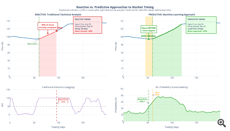
Beyond overfitting, traditional indicator-based approaches suffer from a fundamental timing deficiency. Technical indicators, by construction, are reactive—they process historical data to generate signals after price movements have already begun.

Core Thesis: A truly useful trading system must identify the conditions preceding significant price activity, not the activity itself. The goal is prediction, not confirmation.

This article presents a methodology that synthesizes machine learning research insights into a practical, deployable trading system for XAUUSD (Gold) markets, demonstrated through the "Golden Gauss" architecture.

2. The Core Problems in Algorithmic Trading

2.1 The Overfitting Crisis

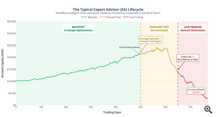
The proliferation of "AI-powered" trading systems in retail markets has created a credibility crisis, with most systems exhibiting catastrophic failure when deployed on unseen data due to severe overfitting.

Figure 1: Conceptual illustration of the typical Expert Advisor lifecycle. Models optimized for historical performance frequently fail catastrophically when deployed on unseen market conditions.

2.2 The Latency Problem in Technical Analysis

Technical indicators are inherently reactive:

• By the time RSI crosses the overbought threshold, the price has already moved significantly
• By the time a MACD crossover confirms, the optimal entry window has passed
• By the time a breakout is "confirmed," stop-loss requirements have expanded substantially

Figure 2: Comparison of timing between reactive technical indicators and predictive machine learning approaches. Traditional indicators confirm moves after optimal entry has passed, while predictive systems identify setup conditions before execution.

2.3 Literature Context

The application of machine learning to financial time-series prediction has evolved substantially. Several consistent findings are relevant:

Finding	Implication
Gradient Boosting Dominance on Tabular Data	Despite marketing appeal of "deep learning," ensemble methods consistently outperform neural networks on structured financial data
Feature Engineering Criticality	Quality of engineered features typically determines model success more than architectural choices
Temporal Validation Requirements	Standard cross-validation that shuffles data is inappropriate for financial time-series due to lookahead bias
Cross-Asset Information	Financial instruments do not trade in isolation; correlated instruments provide valuable context

3. Methodology

3.1 The Predictive Labeling Methodology

Standard approaches to training trading models label data at the point where price movement occurs. This creates a fundamental problem: if the model learns features calculated from the same bars that are labeled, it effectively learns to recognize moves that are already happening rather than moves that are about to happen.

The Golden Gauss architecture employs a methodology that maintains temporal separation between feature calculation and label placement:

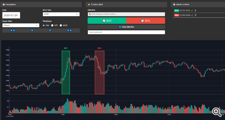
• The labeling process identifies profitable zones where price moved significantly in a specific direction
• All features are calculated from market data that occurred before the labeled zone begins

Figure 3: Manual labeling interface showing XAUUSD price action with identified directional zones. The labeled BUY and SELL regions represent profitable moves used as training targets; the model learns to predict these moves using features calculated from preceding market data.

Implications: This temporal separation ensures the model learns to recognize preconditions—the market microstructure patterns that precede significant moves—rather than characteristics of the moves themselves.

3.2 Quality-Filtered Training Labels

Not all price movements are meaningful or tradeable. Many are:

• Too small to overcome transaction costs (spread + commission)
• Too erratic to execute cleanly
• Part of larger consolidation patterns without directional follow-through

The labeling process applies strict filtering criteria, identifying only zones where price moved with sufficient magnitude and directional consistency. This ensures the model learns exclusively from setups that exceeded minimum profitability thresholds.

3.3 Dual-Model Directional Architecture

Market dynamics exhibit fundamental asymmetry between bullish and bearish behavior:

• Accumulation patterns differ structurally from distribution patterns
• Fear-driven selling typically executes faster than greed-driven buying
• Support behavior differs from resistance behavior
• Volume characteristics differ between advances and declines

To respect this asymmetry, the architecture employs two independent binary models:

Model	Output	Training Data
BUY Model	P(Bullish Move Imminent)	Trained exclusively on bullish labels
SELL Model	P(Bearish Move Imminent)	Trained exclusively on bearish labels

Each model is a binary classifier detecting only its respective directional setup. This prevents the confusion that occurs when a single model attempts to learn contradictory patterns simultaneously.

3.4 Walk-Forward Validation Protocol

Standard machine learning cross-validation, which shuffles data randomly, is inappropriate for financial time-series due to temporal dependencies and lookahead bias risks.

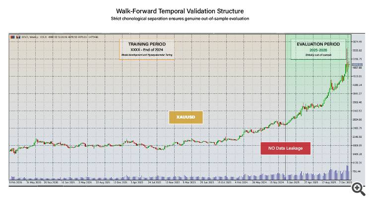
The system uses strict walk-forward validation with complete chronological separation:

• Training data extends through December 31, 2024
• All architectural decisions, hyperparameters, and feature engineering choices were finalized using only this data
• The model was then frozen and validated on a 13-month out-of-sample period (January 2025 through January 2026)

Figure 4: Temporal data separation for walk-forward validation. Training data extends through end of 2024; all 2025-2026 evaluation represents strictly out-of-sample performance on data not used for training.

Critical Rules:

• No shuffling of time-series data
• Evaluation period assessment only after all model decisions finalized
• No iterative "peeking" at evaluation results to adjust parameters

4. System Architecture

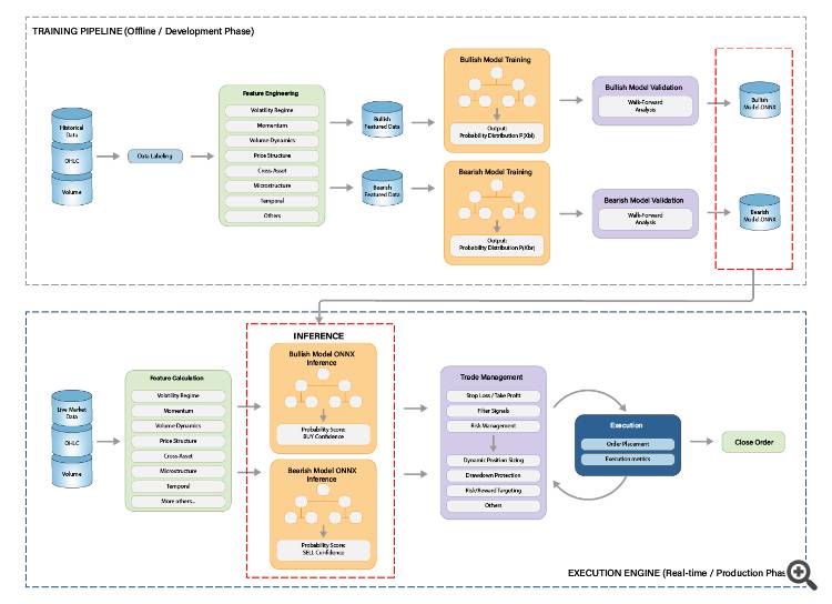
The system comprises two distinct but integrated components:

1. Training Pipeline — implemented in Python for model development and validation
2. Execution Engine — implemented in MQL5 for real-time deployment within MetaTrader 5

Figure 5: High-level architecture of the system. The training pipeline (top) processes historical data through feature engineering and model training, exporting via ONNX. The execution engine (bottom) calculates features instantaneously, obtains probability scores, and applies trade management logic for position execution.

4.1 Model Architecture Selection

The choice of model architecture was driven by empirical evaluation against criteria specific to financial time-series prediction:

Criterion	Priority
Performance on structured/tabular data	Critical
Robustness to noise and outliers	Critical
Handling of regime changes	High
Training data efficiency	High
Inference speed for live deployment	High
Interpretability (feature importance)	Medium

Based on extensive testing, Gradient Boosting Decision Trees (GBDT) were selected. This choice aligns with consistent findings in the machine learning literature that GBDT architectures outperform deep learning approaches on structured financial data.

Why Not Neural Networks?

While "Neural Network" generates marketing appeal, the technical reality for tabular financial data:

• GBDTs handle feature interactions naturally without explicit specification
• GBDTs are more robust to noise and outliers in financial data
• GBDTs require substantially less training data
• GBDTs provide interpretable feature importance rankings
• GBDTs train faster, enabling more extensive hyperparameter search

4.2 ONNX Deployment

The model is exported via ONNX (Open Neural Network Exchange) for platform-agnostic deployment, enabling Python-trained models to execute at C++ speeds within MT5.

A critical requirement is training-serving parity: feature calculations in MQL5 must be mathematically identical to those performed during Python training. Any discrepancy creates "training-serving skew" that degrades model performance.

4.3 The MQL5-ONNX Interface

The bridge between Python training and MQL5 execution relies on the native ONNX API introduced in MetaTrader 5 Build 3600. The primary engineering challenge is ensuring the input tensor shape matches the Python export exactly, and correctly interpreting the classifier's dual-output structure.

Below is the structural logic used to initialize and run inference with the Gradient Boosting model within the Expert Advisor:

Model Initialization

#resource "\\Files\\BULLISH_Model.onnx" as uchar ExtModelBuy[]
long g_onnx_buy;
const int SNIPER_FEATURES = 239;

bool InitializeONNXModels()
{
    Print("Loading ONNX models...");
    
    // Load BUY model
    g_onnx_buy = OnnxCreateFromBuffer(ExtModelBuy, ONNX_DEFAULT);
    if(g_onnx_buy == INVALID_HANDLE)
    {
        Print("[FAIL] Failed to load BUY model");
        return false;
    }
    
    // Set input shape for BUY model
    ulong input_shape_buy[] = {1, SNIPER_FEATURES};
    if(!OnnxSetInputShape(g_onnx_buy, 0, input_shape_buy))
    {
        Print("[FAIL] Failed to set BUY model input shape");
        return false;
    }
    
    Print("   [OK] BUY model loaded successfully");
    return true;
}

Probability Inference

The classifier outputs two tensors: predicted labels and class probabilities. For probability-based execution, we extract the probability of the target class:

bool GetBuyPrediction(const float &features[], double &probability)
{
    probability = 0.0;
    
    if(g_onnx_buy == INVALID_HANDLE)
    {
        Print("[FAIL] BUY model not loaded");
        return false;
    }
    
    // Prepare input (239 features)
    float input_data[];
    ArrayResize(input_data, SNIPER_FEATURES);
    ArrayCopy(input_data, features);
    
    // Classifier has 2 outputs:
    // Output 0: predicted label (int64) - shape [1]
    // Output 1: class probabilities (float32) - shape [1, 2]
    
    long output_labels[];      // Predicted class label
    float output_probs[];      // Class probabilities [P(class0), P(class1)]
    
    ArrayResize(output_labels, 1);
    ArrayResize(output_probs, 2);
    ArrayInitialize(output_labels, 0);
    ArrayInitialize(output_probs, 0.0f);
    
    // Run inference with both outputs
    if(!OnnxRun(g_onnx_buy, ONNX_NO_CONVERSION, input_data, output_labels, output_probs))
    {
        int error = GetLastError();
        Print("[FAIL] BUY ONNX inference failed: ", error);
        return false;
    }
    
    // output_probs[0] = probability of BULLISH (class 0)
    // output_probs[1] = probability of NOT-BULLISH (class 1)
    probability = (double)output_probs[0];
    
    return true;
}

Key Implementation Details:

• Dual-Output Structure: Gradient Boosting classifiers exported via ONNX produce two outputs—the predicted label and the probability distribution across classes. The probability output is used for threshold-based execution.
• Class Mapping: Class 0 represents the target condition (BULLISH for the BUY model). The probability output_probs[0] directly indicates model confidence in an imminent bullish move.
• Shape Validation: Strict shape checking at initialization catches training-serving mismatches immediately rather than producing silent prediction errors during live trading.

4.4 Execution Configuration

Parameter	Value
Symbol	XAUUSD only
Timeframe	M1 (feature calculation)
Active Hours	14:00–18:00 (broker time, configurable)
Probability Threshold	88%
Stop Loss	Fixed initial; dynamically managed
Take Profit	Target-based with ratchet protection
Prohibited Strategies	No grid, no martingale

5. Feature Engineering

The system processes 239 engineered features across multiple research-backed domains. These features were developed through academic literature review, domain expertise in market microstructure, and iterative empirical testing with strict validation protocols.

5.1 Feature Categories Overview

Category	Conceptual Focus
Volatility Regime	Market state classification, tradeable vs. non-tradeable conditions
Momentum	Multi-scale rate of change, trend persistence
Volume Dynamics	Participation levels, unusual activity detection
Price Structure	Support/resistance proximity, range position
Cross-Asset	Correlated instrument signals, correlation regime shifts
Microstructure	Directional pressure and short-horizon stress proxies
Temporal	Session timing, cyclical patterns
Sequential	Pattern recognition, run-length analysis

5.2 Key Driving Features

The following features consistently ranked among the most influential according to global SHAP importance analysis:

• ADX Trend Strength (14-period): Measuring trend strength, independent of direction
• VWAP Volatility Deviation: Distance of price from intraday VWAP, normalized by recent volatility
• Volatility Regime Classifier: ATR relative to its moving average, indicating low-, normal-, or high-volatility states
• MACD Histogram Momentum: Capturing short-term momentum and potential reversals
• 60-minute Gold/DXY Rolling Correlation: Rolling correlation between XAUUSD and DXY returns
• 60-minute Gold/USDJPY Rolling Correlation: Rolling correlation between XAUUSD and USDJPY returns
• Directional Volatility Regime: Signed volatility feature combining EMA-based trend strength with current ATR regime
• Order-Flow Persistence: Proxy for how long directional moves persist across recent candles
• EMA Spread Dynamics: Distances and slopes between fast and slow EMAs

The presence of well-known indicators (ADX, MACD) alongside proprietary regime and correlation features demonstrates that the model enhances, rather than replaces, established market relationships with higher-resolution timing signals.

5.3 Cross-Asset Intelligence

Gold (XAUUSD) does not trade in isolation. Its price action is influenced by:

• US Dollar Dynamics: Typically inverse correlation; dollar strength generally pressures gold prices
• Safe-Haven Flows: Correlation with other safe-haven assets during risk-off periods
• Yield Expectations: Relationship with real interest rate proxies

The feature set incorporates lagged returns from correlated instruments, rolling correlations at multiple time scales, divergence detection, and regime change signals.

6. Validation and Results

The validation approach follows a single principle: demonstrate generalization, not memorization. Any model can achieve spectacular results on data it has seen. The only meaningful evaluation is performance on strictly unseen data.

6.1 Out-of-Sample Performance

All 2025 performance represents true out-of-sample (OOS) results. The model architecture, hyperparameters, and feature set were frozen before any 2025 data was evaluated.

Figure 6: Backtest equity and balance curves from Jan 2021 to Jan 2026. The period Jan 2021–Dec 2024 represents data included in model training; the period Jan 2025–Jan 2026 constitutes strictly out-of-sample evaluation.

Metric	Full Period (Jan 2021– Jan 2026)	OOS Only (Jan 2025–Jan 2026)
Win Rate	88.71%	83.67%
Total Trades	1,030	319
Profit Factor	1.77	1.50
Sharpe Ratio	9.90	13.9
Max Drawdown (0.01 lot)	~$500	~$313
Recovery Factor	11.57	3.66
Avg Holding Time	30 min 30 sec	30 min 30 sec

Interpretation: The out-of-sample period demonstrates continued profitability with metrics that degrade gracefully from the training period:

• Win rate decreases from 88.71% to 83.67%—a controlled 5% reduction indicating the model generalizes rather than memorizes
• Profit factor remains above 1.50, confirming positive expectancy on unseen data
• The higher OOS Sharpe ratio (13.9 vs 9.90) provides strong evidence against overfitting

This performance gap is expected and healthy. The controlled degradation confirms genuine pattern generalization.

6.2 Probability Threshold Analysis

The model outputs continuous probability scores. Analysis reveals the relationship between probability levels and trade outcomes:

Probability Range	Trades	Win Rate
0.880 – 0.897	231	88.3%
0.897 – 0.923	167	90.4%
0.923 – 0.950	190	93.2%
0.950 – 0.976	107	87.9%
0.976 – 0.993	27	96.3%

Why 88% Minimum Threshold? The 88% threshold was determined through systematic evaluation as the optimal entry point balancing trade frequency against quality. Below this threshold, false-positive rates increase significantly.

6.3 Exit Composition Analysis

Exit Type	Percentage	Interpretation
Ratchet Profit (SL_WIN)	87.1%	Dynamic profit capture
Take Profit (TP)	3.2%	Full target reached
Stop Loss (SL_LOSS)	9.7%	Controlled losses

The vast majority of winning trades exit via the ratchet system, capturing profits dynamically rather than waiting for full TP.

6.4 Temporal Consistency

Year	Trades	Win Rate	Status
2021	172	93.6%	Training
2022	125	93.6%	Training
2023	64	87.5%	Training
2024	124	93.5%	Training
2025	237	85.2%	Out-of-Sample
2026	---	---	---

All years profitable with consistent performance patterns across training and out-of-sample periods.

7. Trade Management

The system implements a comprehensive trade management layer that extends beyond simple entry execution.

7.1 Probability-Based Decision Making

Unlike systems that generate discrete "buy" or "sell" signals, the architecture calculates probability scores instantaneously on each new bar:

• Entry Decision: Probability must exceed 88% threshold before position opening
• Direction Selection: Higher probability between BUY and SELL models determines direction
• Exit Timing: Probability changes inform position closure decisions
• Hold/Close Logic: Continuous probability monitoring during open positions

7.2 Entry Validation and Filtering

• Dual-Model Confirmation: Both BUY and SELL model probabilities are assessed to confirm directional bias and filter ambiguous conditions
• Regime Filtering: Additional filters detect unfavorable market regimes (high volatility events, low liquidity periods)
• Conditional Execution: Trade execution proceeds only after probability thresholds are satisfied and regime filters confirm favorable conditions

7.3 Ratchet Profit Protection

Problem Addressed: Price may move 80% toward the take-profit level, then reverse—without active management, this unrealized profit would be lost.

Ratchet Solution: As price moves favorably, the system progressively locks in profit by tightening exit conditions, ensuring that significant favorable moves are captured even if the full take-profit is not reached.

7.4 Ratchet Loss Minimization

Problem Addressed: Even high-confidence predictions occasionally fail; waiting for the fixed stop-loss results in maximum loss on every losing trade.

Ratchet Solution: When price moves adversely, the system actively manages the exit to minimize loss rather than passively waiting for stop-loss execution, reducing average loss per unsuccessful trade.

8. Honest Limitations

8.1 What This System Is NOT

• Not infallible: Approximately 15–18% of signals result in suboptimal entries depending on market conditions
• Not universal: Trained exclusively for XAUUSD with its specific market microstructure and session dynamics
• Not static: Periodic retraining (3–6 months) is required as markets evolve
• Not guaranteed: Out-of-sample validation demonstrates methodology soundness but does not guarantee future performance

8.2 Identified Risk Factors

Risk	Description	Mitigation
Regime Change	Market structure evolves through policy shifts and geopolitical events	Periodic retraining protocol
Execution Risk	Slippage during volatility can degrade realized results	Session-aware execution, active hours restriction
Edge Decay	Predictive edges face decay as markets evolve	Retraining with methodology preservation
Concentration	Exclusive XAUUSD focus provides no diversification	User responsibility for portfolio allocation

8.3 Execution Assumptions

All reported results are based on historical simulations. No additional slippage model has been applied, and real-world execution may lead to materially different performance. These statistics should be interpreted as estimates under ideal execution conditions.

9. Conclusion

This article presented a methodology for solving two fundamental failures that characterize retail algorithmic trading—overfitting to historical noise and reactive signal generation—through rigorous machine learning practices.

The core innovations demonstrated in the Golden Gauss architecture include:

• Predictive labeling that enables genuine anticipation of price moves
• Dual-model directional specialization that respects market asymmetry
• Probability-driven execution that quantifies confidence before trade entry
• Intelligent trade management that minimizes losses when predictions prove suboptimal

On strictly out-of-sample 2025 data—collected after all model decisions were finalized—the system demonstrates approximately 83.67% directional accuracy at the 88% probability threshold. The controlled performance differential from training metrics indicates genuine pattern learning rather than memorization.

Key Takeaways for Practitioners

1. Never shuffle time-series data during validation—this creates lookahead bias and data leakage
2. Out-of-sample performance is the only meaningful metric for evaluating live trading potential
3. Probability thresholds enable accuracy/frequency tradeoffs—higher thresholds yield fewer but higher-quality signals
4. Dual binary models respect the asymmetry between bullish and bearish market dynamics
5. Trade management amplifies edge—ratchet mechanisms maximize wins and minimize losses
6. All systems have limitations—honest acknowledgment enables appropriate deployment and risk management

The retail algorithmic trading industry suffers from systematic misalignment between vendor incentives and user outcomes. The methodology presented here—strict temporal separation, documented performance degradation, bounded confidence claims—offers a template for honest system evaluation that prioritizes sustainable operation over marketing appeal.

Expert critique of the validation methodology and underlying assumptions is welcomed. Progress in algorithmic trading requires systems designed to survive scrutiny rather than avoid it.

10. Implementation & Availability

The architecture described in this paper—specifically the predictive labeling engine and the ONNX probability inference—has been fully implemented in the Golden Gauss AI system.

To support further research and validation, the complete system is available for testing in the MQL5 Market. The package includes the "Visualizer" mode, which renders the probability cones and "Kill Zones" directly on the chart, allowing traders to observe the model's decision-making process in real-time.

• Expert Advisor: Golden Gauss AI (MQL5 Market)
• Research Paper: Full Methodology (Zenodo)

Risk Disclaimer: Trading forex and CFDs involves substantial risk of loss and is not suitable for all investors. Past performance, whether in backtesting or live trading, does not guarantee future results. The validation results presented represent historical analysis under specific market conditions that may not persist. Traders should only use capital they can afford to lose and should consider their financial situation before trading.

References

1. Cao, L. J. and Tay, F. E. H. (2001). Financial forecasting using support vector machines. Neural Computing & Applications, 10(2), 184-192.
2. Chen, T. and Guestrin, C. (2016). XGBoost: A scalable tree boosting system. Proceedings of the 22nd ACM SIGKDD International Conference on Knowledge Discovery and Data Mining, 785-794.
3. López de Prado, M. (2018). Advances in Financial Machine Learning. Wiley.
4. Bailey, D. H. and López de Prado, M. (2014). The probability of backtest overfitting. Journal of Computational Finance, 17(4), 39-69.
5. Pardo, R. (2008). The Evaluation and Optimization of Trading Strategies (2nd ed.). Wiley.
6. Krauss, C., Do, X. A., and Huck, N. (2017). Deep neural networks, gradient-boosted trees, random forests: Statistical arbitrage on the S&P 500. European Journal of Operational Research, 259(2), 689-702.
7. Baur, D. G. and McDermott, T. K. (2010). Is gold a safe haven? International evidence. Journal of Banking & Finance, 34(8), 1886-1898.
8. ONNX Runtime Developers (2021). ONNX Runtime: High performance inference and training accelerator. Available: https://onnxruntime.ai/