
Fundamentals of Statistics

Introduction
What is statistics? Here is the definition found on Wikipedia: "Statistics is the study of the collection, organization, analysis, interpretation, and presentation of data." (Statistics). This definition suggests three main components of statistics: data collection, measurement and analysis. Data analysis appears to be especially useful for a trader as information received is provided by the broker or via a trading terminal and is already measured.
Modern traders (mostly) use technical analysis to decide whether to buy or sell. They deal with statistics in virtually everything they do when using a certain indicator or trying to predict the level of prices for the upcoming period. Indeed, a price fluctuation chart itself represents certain statistics of a share or currency in time. It is therefore very important to understand the basic principles of statistics underlying the majority of mechanisms that facilitate the decision making process for a trader.
Probability Theory and Statistics
Any statistics is the result of change in the states of the object that generates it. Let us consider a EURUSD price chart on hourly time frames:

In this case, the object is the correlation between two currencies, while the statistics is their prices at every point of time. How does the correlation between two currencies affect their prices? Why do we have this price chart and not a different one at the given time interval? Why are the prices currently going down and not up? The answer to these questions is the word 'probability'. Every object, depending on probability, can take one or another value.
Let us do a simple experiment: take a coin and flip it a certain number of times, every time recording the toss outcome. Suppose we have a fair coin. Then the table for it can be as follows:
| Outcome | Probability |
|---|---|
| Heads | 0.5 |
| Tails | 0.5 |
The table suggests that the coin is equally likely to come up heads or tails. Any other outcome is not possible here (landing on the coin's edge has been excluded a priori) as the sum of probabilities of all possible events shall be equal to one.
Flip the coin 10 times. Now let us look at the toss outcomes:
| Outcome | Number |
|---|---|
| Heads | 8 |
| Tails | 2 |
Why do we have these results if the coin is equally likely to land on either of the sides? The probability of the coin to land on either of the sides is indeed equal, which however does not mean that after a few tosses the coin shall land on one side as many times as on the other side. The probability only shows that in this particular attempt (toss) the coin will land either heads up or tails up and both events stand equal chances.
Let us now flip the coin 100 times. We get the new table of outcomes:
| Outcome | Number |
|---|---|
| Heads | 53 |
| Tails | 47 |
As can be seen, the numbers of outcomes are again not equal. However, 53 to 47 is the result that proves the initial probability assumptions. The coin landed on heads in nearly as many flips as it did on tails.
Now let us do the same in the reverse order. Suppose we have a coin but the probability of landing on its sides is unknown. We need to determine if it is a fair coin, i.e. the coin that is equally likely to come up heads or tails.
Let us take the data from the first experiment. Divide the number of outcomes per side by the total number of outcomes. We get the following probabilities:
| Outcome | Probability |
|---|---|
| Heads | 0.8 |
| Tails | 0.2 |
We can see that it is very difficult to conclude from the first experiment that the coin is fair. Let us do the same for the second experiment:
| Outcome | Number |
|---|---|
| Heads | 0.53 |
| Tails | 0.47 |
Having these results at hand, we can say with a high degree of accuracy that this is a fair coin.
This simple example allows us to draw an important conclusion: the bigger the number of experiments, the more accurately the object properties are reflected by statistics generated by the object.
Thus, statistics and probability are inextricably intertwined. Statistics represents experimental results with an object and is directly dependent on probability of the object states. Conversely, the probability of the object's states can be estimated using statistics. Here is where the main challenge for a trader lies: having data on trades over a certain period of time (statistics), to predict the price behavior for the following period of time (probability) and based on this information to make a buy or sell decision.
Therefore, getting back to the points made in Introduction, it is also important to know and understand the relationship between statistics and probability, as well as to have knowledge of risk assessment and risk situations. The latter two are however out of the scope of this article.
Basic Statistical Parameters
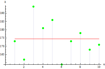
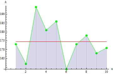
Let us now review the basic statistical parameters. Suppose we have data on height in cm regarding 10 people in a group:
| 1 | 2 | 3 | 4 | 5 | 6 | 7 | 8 | 9 | 10 | |
|---|---|---|---|---|---|---|---|---|---|---|
| Height | 173 | 162 | 194 | 181 | 186 | 159 | 173 | 178 | 168 | 171 |
The data set forth in the table is called sample, while the data quantity is the sample size. We will take a look at some parameters of the given sample. All parameters will be sample parameters as they result from the sample data, rather than random variable data.
1. Sample mean
Sample mean is the average value in the sample. In our case, it is the average height of people in the group.
To calculate the mean, we should:
- Add up all sample values.
- Divide the resulting value by the sample size.
Formula:
![]()
Where:
- M is the sample mean,
- a[i] is the sample element,
- n is the sample size.
Following the calculations, we get the mean value of 174.5 cm
2. Sample variance
Sample variance describes how far sample values lie from the sample mean. The larger the value, the more widely the data is spread out.
To calculate the variance, we should:
- Calculate the sample mean.
- Subtract the mean from each sample element and square the difference.
- Add up the resulting values obtained above.
- Divide the sum by the sample size minus 1.
Formula:
![]()
Where:
- D is the sample variance,
- M is the sample mean,
- a[i] is the sample element,
- n is the sample size.
The sample variance in our case is 113.611.
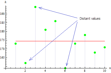
The figure suggests that 3 values are widely spread out of the mean which leads to the large variance value.
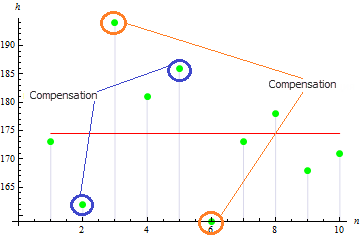
3. Sample skewness
Sample skewness is used for describing the degree of asymmetry of the sample values around its mean. The closer the skewness value is to zero, the more symmetrical the sample values are.
To calculate the skewness, we should:
- Calculate the sample mean.
- Calculate the sample variance.
- Add up cubed differences of each sample element and the mean.
- Divide the answer by the variance value raised to the power of 2/3.
- Multiply the answer by the coefficient equal to the sample size divided by the product of the sample size minus 1 and sample size minus 2.
Formula:
![]()
Where:
- A is the sample skewness,
- D is the sample variance,
- M is the sample mean,
- a[i] is the sample element,
- n is the sample size.
We get a quite small value of skewness for this sample: 0.372981. This is due to the fact that divergent values compensate each other.
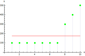
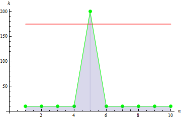
The value will be larger for asymmetrical sample. E.g. the value for the data as below will be 1.384651.
4. Sample kurtosis
Sample kurtosis describes the peakedness of the sample.
To calculate kurtosis, we should:
- Calculate the sample mean.
- Calculate the sample variance.
- Add up the fourth-power differences of each sample element and the mean.
- Divide the answer by the squared variance.
- Multiply the resulting value by the coefficient equal to the product of the sample size and the sample size plus 1, divided by the product of the sample size minus 1, sample size minus 2 and sample size minus 3.
- Subtract from the resulting value the product of 3 and the squared difference of the sample size and 1, divided by the product of the sample size minus 1 and sample size minus 2.
Formula:
![]()
Where:
- E is the sample kurtosis,
- D is the sample variance,
- M is the sample mean,
- a[i] is the sample element,
- n is the sample size.
For the given height data, we get the value of -0.1442285.
For a sharper peak data, we get a larger value: 10.
5. Sample covariance
Sample covariance is a measure indicating the degree of linear dependence between two data samples. Covariance between linearly independent data will be 0.
To illustrate this parameter, we will add weight data for each of the 10 persons:
| 1 | 2 | 3 | 4 | 5 | 6 | 7 | 8 | 9 | 10 | |
|---|---|---|---|---|---|---|---|---|---|---|
| Weight | 65 | 70 | 83 | 60 | 105 | 58 | 69 | 90 | 78 | 65 |
To calculate covariance of two samples, we should:
- Calculate the mean of the first sample.
- Calculate the mean of the second sample.
- Add up all products of two differences: the first difference - an element of the first sample minus the mean of the first sample; the second difference - an element of the second sample (corresponding to the element of the first sample) minus the mean of the second sample.
- Divide the answer by the sample size minus 1.
Formula:
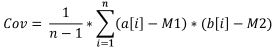
Where:
- Cov is the sample covariance,
- a[i] is the element of the first sample,
- b[i] is the element of the second sample,
- M1 is the sample mean of the first sample,
- M2 is the sample mean of the second sample,
- n is the sample size.
Let us calculate the covariance value of the two samples: 91.2778. The existing dependence can be shown in the combined chart:
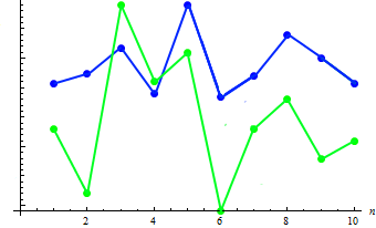
As can be seen, the increase in height (as a rule) corresponds to the decrease in weight and vice versa.
6. Sample correlation
Sample correlation is also used to describe the degree of linear dependence between two data samples but its value always lies within the range of -1 to 1.
To calculate correlation of two samples, we should:
- Calculate the variance of the first sample.
- Calculate the variance of the second sample.
- Calculate covariance of these samples.
- Divide the covariance by the square root of the product of the variances.
Formula:
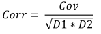
Where:
- Corr is the sample correlation,
- Cov is the sample covariance,
- D1 is the sample variance of the first sample,
- D2 is the sample variance of the second sample,
For the given height and weight data, correlation will be equal to 0.579098.
How to Use Statistics in Trading
The simplest example illustrating the use of statistical parameters in trading is the MovingAverage indicator. Its calculation requires data over a certain period of time and gives the arithmetic mean value of the price:
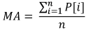
Where:
- MA is the indicator value,
- P[i] is the price,
- n is the MA measurement period
We can see that the indicator is a complete analog of the sample mean. Despite its simplicity, this indicator is used when calculating EMA, the exponential moving average which, in turn, is a basic element required for the MACD indicator - a classical tool for determining the trend strength and direction.

Statistics in MQL5
We will look at the MQL5 implementation of the basic statistical parameters described above. The statistical methods reviewed above (and a lot more) are implemented in the statistical functions library statistics.mqh. Let us review their codes.
1. Sample mean
The library function calculating the sample mean is called Average:

Input data: data sample. Output data: mean.
2. Sample variance
The library function calculating the sample variance is called Variance:

Input data: data sample and its mean. Output data: variance.
3. Sample skewness
The library function calculating the sample skewness is called Asymmetry:

Input data: data sample, its mean and variance. Output data: skewness.
4. Sample kurtosis
The library function calculating the sample kurtosis is called Excess (Excess2):

Input data: data sample, its mean and variance. Output data: kurtosis.
5. Sample covariance
The library function calculating the sample covariance is called Cov:

Input data: two data samples and their respective means. Output data: covariance.
6. Sample correlation
The library function calculating the sample correlation is called Corr:

Input data: covariance of two samples, variance of the first sample and variance of the second sample. Output data: correlation.
Let us now input height and weight sample data and process it using the library.#include <Statistics.mqh> //+------------------------------------------------------------------+ //| Script program start function | //+------------------------------------------------------------------+ void OnStart() { //--- specify two data samples. double arrX[10]={173,162,194,181,186,159,173,178,168,171}; double arrY[10]={65,70,83,60,105,58,69,90,78,65}; //--- calculate the mean double mx=Average(arrX); double my=Average(arrY); //--- to calculate the variance, use the mean value double dx=Variance(arrX,mx); double dy=Variance(arrY,my); //--- skewness and kurtosis values double as=Asymmetry(arrX,mx,dx); double exc=Excess(arrX,mx,dx); //--- covariance and correlation values double cov=Cov(arrX,arrY,mx,my); double corr=Corr(cov,dx,dy); //--- print results in the log file PrintFormat("mx=%.6e",mx); PrintFormat("dx=%.6e",dx); PrintFormat("as=%.6e",as); PrintFormat("exc=%.6e",exc); PrintFormat("cov=%.6e",cov); PrintFormat("corr=%.6e",corr); }
After executing the script, the terminal will produce the results as follows:
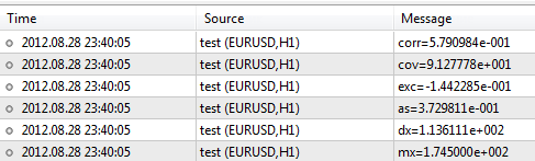
The library contains a lot more functions the descriptions of which can be found in CodeBase - https://www.mql5.com/en/code/866.
Conclusion
Some conclusions have already been drawn at the end of the "Probability Theory and Statistics" section. In addition to the above, it would be worth mentioning that statistics, like any other branch of science, shall be studied starting with its ABCs. Even its basic elements can facilitate the understanding of a great deal of complex things, mechanisms and patterns which at the end of the day can be extremely necessary in trader's work.
Translated from Russian by MetaQuotes Ltd.
Original article: https://www.mql5.com/ru/articles/387
Warning: All rights to these materials are reserved by MetaQuotes Ltd. Copying or reprinting of these materials in whole or in part is prohibited.
This article was written by a user of the site and reflects their personal views. MetaQuotes Ltd is not responsible for the accuracy of the information presented, nor for any consequences resulting from the use of the solutions, strategies or recommendations described.

 Exploring Trading Strategy Classes of the Standard Library - Customizing Strategies
 How to purchase a trading robot from the MetaTrader Market and to install it?
 Automata-Based Programming as a New Approach to Creating Automated Trading Systems
 MetaQuotes ID in MetaTrader Mobile Terminal
- Free trading apps
- Over 8,000 signals for copying
- Economic news for exploring financial markets
You agree to website policy and terms of use
There should be plenty of algorithms for determining mods, so a universal bicycle is not useful here.
You should rather look at examples, what you want to get and what you don't want to get.
I liked the article.
It is very easy to understand and contains enough information.
And, judging by the title, it doesn't pretend to be more than that.
I don't see any use for this article. A number of platitudes from TV. And if this article was not printed on a specialised, half-trader website, it would be possible to keep silent. But considering the site, I would like to note the following.
There is a science of measuring, analysing and forecasting economic data. It is called econometrics. It is a close, blood relative of statistics, but there are significant differences.
1. For traders, the analysis itself has no value if the forecast does not follow from the analysis. The article does not mention forecasting at all.
2. Econometrics initially proceeds from the non-stationarity of economic series. And if one would at least remember about it, keep it in mind, so to speak, the story about basic statistics would not be so rosy: for non-stationary series the basic concepts of mo, variance, etc. can be applied with a lot of reservations. At any rate one should always be in doubt. For example, for non-stationary series, the mean will not necessarily converge to the mo. I am not talking about correlation at all.
3. econometrics is based on very short samples - a few dozens of observations. It is not interested in the average for many years, since such an average also implies being in a pose for several years. In crises, estimates of the results of the calculation become important. It is the estimates that radically distinguish TV from statistics and especially from econometrics.
School article. The level of a special school, not even junior courses of an institute.
"From this simple example, we can draw an important conclusion: as the number of trials increases, statistics more accurately reflects the properties of the object that generates them."
For a stationary process (Spherical Horse in Vacuum) - Yes.
For Time Series of real data this statement is more like nonsense.
If Forex were a Stationary Time Series - MQL5 would not be needed to estimate it - simple wooden brushes from the grocery store would suffice.
If holes are drilled in the moth in a chaotic order and at chaotic time intervals.
then the statistics for the whole period will be more like a RosStat report - or the ravings of a madman.
"This is where the main task of a trader arises: knowing the data on trades for a certain period of time (statistics), predict the behaviour of prices (rate) for the next period of time (get probability), and based on this make a decision to buy or sell."
another statement in terms of meaning is not far from nonsense. In order to forecast something, one should first prove to oneself that the series is not random and can be forecasted. It is possible to have income on random series. they cannot be predicted but you can get out of them. probability asymmetry and positive/negative expectation.
.