Change Point Detection for Financial Time Series in MQL5
 98
 0

Introduction
Financial returns do not behave the same way throughout a history. A market that trends smoothly for months may move into a highly volatile phase after an announcement, and the mean and variance of its returns can shift with it. The task in this article is to divide a return history into segments with different mean and variance, in a repeatable way, and to ask at which points the modeled behavior of returns changed enough that treating them as one continuous regime stops being a good fit.
The solution combines a Gaussian segment cost, a fixed penalty per change point, and the Pruned Exact Linear Time (PELT) algorithm, implemented as four cooperating MQL5 classes. PELT finds the optimal segmentation exactly, discarding candidate break points once they can no longer be optimal, provided a condition on the cost holds, which the script checks before it prunes.
The limitations matter enough to state at the start:
- The method is retrospective. It marks up history and is not a trading signal. Because each segment must be at least a minimum length, it cannot report a change point in the last few bars, and change points near the end of the window can shift when new data arrives.
- It is not a hypothesis test. "Statistical" here means derived from a Gaussian mean-and-variance segmentation model with a given penalty. There is no p-value or confidence level behind any individual break.
- Repeatable does not mean assumption-free. The same data and settings always give the same answer, but the cost function, the penalty and the minimum segment length are choices, and different choices give different segmentations.
Understanding Change Point Detection
Time series. Here it is the sequence of logarithmic returns computed from historical closing prices, ordered by time. Detection is applied to returns, not to raw prices.
Structural break (change point). Throughout this article, a structural break, or change point, means a point where the segmentation model prefers to start a new segment, because a Gaussian with its own mean and variance on each side fits the data better than a single Gaussian would, by more than the penalty. This is a statement about the model's objective. It is not a claim that something happened in the market, and a real market event may or may not produce one.
Segmentation. Once one or more change points are found, the time series is naturally divided into contiguous segments. Each segment is modeled as homogeneous, that is, generated by a single, unchanging return distribution.
The method looks for changes in the mean return, the variance, or both. These changes can accompany news events, crises and recovery periods. However, a detected boundary only indicates an improvement in the quality of the split under the selected model. It does not identify the cause of the change.
The Mathematics Behind Change Point Detection
Segmenting a time series
Suppose we have returns y_1, ..., y_n. A segmentation is a set of change points 0 = t_0 < t_1 < ... < t_m = n that splits the series into m contiguous segments. The cost function C(s, e) scores how badly a single Gaussian, with its own mean and variance, fits the returns between indices s and e. Pooling two different regimes into one segment inflates the variance and the cost.
C(s, e) = n * ln(var)
Here var is the maximum-likelihood variance of the segment: the sum of squared deviations from the segment mean divided by n, not n - 1. The cost is -2 ln L of the fitted Gaussian with the constants dropped that are identical for every segmentation, since the total number of observations is fixed.
If every return in a segment is identical, the variance is zero and ln(0) diverges, so the cost needs a floor:
C(s, e) = n * ln(max(var, ε)), ε = 10⁻⁸ × var_all var_all is the variance of the entire return series, so the floor scales with the data and the segmentation does not change under rescaling of the returns. The floor is part of the objective, so whenever we call the solution "exact" below, we mean exact for this floored objective. In practice ε only binds on near-constant segments, such as runs of identical closes.
Objective and recursion
The total cost of a segmentation is the sum of its segment costs plus a penalty β per change point. Minimizing it is the optimal partitioning problem, solved by dynamic programming:
Total cost = Σ C(t_(k-1), t_k) + (m - 1)·β
F(t) = min over τ < t of [F(τ) + C(τ, t) + β],   F(0) = -β
F(t) is the minimum total cost of segmenting the first t observations, and the τ that achieves each minimum is stored so the change points can be recovered by walking back from F(n). Setting F(0) = -β cancels the penalty that the recursion would otherwise charge for the first segment. A prefix shorter than one minimum segment length has no legal segmentation at all, and the implementation tracks this explicitly instead of forcing an answer.

Choosing the penalty
Adding change points always lowers the fit cost, in the same way that adding parameters to a regression always lowers the residual error, so a fixed penalty β per change point is needed. If β is too small the algorithm chases noise, and if it is too large genuine shifts are smoothed over.
The cost above is already on the -2 ln L scale. As an initial calibration we use a BIC-style penalty, β = 2·ln(n), which corresponds to two additional parameters per segment, the mean and the variance. It is applied automatically when InpPenalty is zero or negative. This is not a universal calibration: counting the break position as a parameter would push the multiplier toward 3, and other ways of accounting for data complexity and properties may require a larger penalty. Treat β as a setting to examine, which is what the sensitivity scan later in the article is for.
The PELT pruning ruleA direct implementation of the recursion is O(n²), because every endpoint t checks every earlier τ. PELT removes most of that work with one observation. If at endpoint t a candidate τ satisfies F(τ) + C(τ, t) > F(t), then τ can never be the best last change point for any later endpoint T:
F(τ) + C(τ, T) + β ≥ F(τ) + C(τ, t) + C(t, T) + β > F(t) + C(t, T) + β
The first step relies on one property of the cost: splitting a segment never makes the total worse, C(τ, t) + C(t, T) ≤ C(τ, T). The unfloored Gaussian cost has that property, so τ can be discarded for good. Under the conditions in the PELT literature the expected running time is close to linear, though the worst case remains O(n²). Pruning never changes the answer, only the amount of work.
Minimum segment length and deferred removal. With a minimum length m, t is only a legal last change point for endpoints T ≥ t + m. Between t and t + m, swapping τ for t would create a segment that is too short, so τ may still be the best choice. The fix is to postpone the removal: when τ first satisfies the inequality at t, we mark it and keep it active until endpoint t + m, then drop it. Dropping it immediately can return a segmentation that is slightly worse than the true optimum.
Randomized testing supports this. We compared three pruning variants with a brute-force partitioner that tries every admissible τ: immediate removal, deferred removal, and deferred removal combined with the check described below. The test used 2,400 simulated series (fixed seed, lengths 40 to 200 returns, minimum segment lengths 2 to 15). Immediate pruning produced a different segmentation from brute force on 74 of them. Both deferred variants matched on all 2,400. On a 500-return series with a minimum length of 10, pruning reduced the number of segment cost evaluations from 116,412 to 33,153, with identical change points. The check switched pruning off on 532 of the 2,400 series, mostly those with runs of identical or near-identical closes, so on those series the solver ran the full recursion. The test setup is described in Appendix A.A caveat for the floored cost. The inequality holds exactly for the unfloored Gaussian cost, but it can fail once the ε floor binds. Take two adjacent segments of equal length k with the same mean, where the first is constant, so its variance is floored to ε, and the second has variance 2ε. Together they have variance ε, so the merged segment costs 2k·ln ε, while the two pieces cost k·ln ε + k·ln 2ε, which is larger by k·ln 2. Splitting made the total worse, so for the floored cost the pruning argument is not guaranteed in general. A matching result in randomized tests is not a proof, and a stress test with a binding floor shows why the check is needed: without it, deferred pruning gave a different segmentation from brute force on 30 of 29,814 series, while the guarded version never did.
The script therefore prunes only when it can verify a sufficient condition. Every segment in the pruning argument has at least m returns, so if no segment of m or more returns has a variance below ε, the floor never binds and the unfloored inequality applies. It is enough to check windows of exactly m returns: any longer segment can be cut into blocks of m to 2m - 1 returns, and a block's variance is more than half the variance of its first m returns. If the smallest m-window variance is at least 2ε, every admissible segment sits above the floor. If the check fails, for instance on a long run of identical closes, the solver runs the full recursion with no pruning, which is slower but exact for the floored objective by construction.
Minimum segment length
A segment containing a single return has zero variance, so its cost is clamped to the floor, and the optimizer finds that cutting the series into single-return pieces makes every segment look perfectly fitted. On five simulated series of 500 pure-noise returns with a minimum length of 1, the segmentation returned between 496 and 499 change points. The script therefore rejects any InpMinSegmentLength below 2, and we recommend 5 to 10. The default of 10 is inside that range, and as long as the pruning check above passes, it runs genuine PELT.
Designing the Change Point Detection Framework
With the theory in place, the implementation is organized into four cooperating classes, each with a single, clear responsibility:
| Class | Responsibility |
|---|---|
| CChangePointModel | Downloads price history, computes log returns, and builds the cumulative statistics arrays used for fast segment evaluation. |
| CSegmentCost | Computes the Gaussian mean/variance cost C(s, e) for any candidate segment, using the cumulative statistics from CChangePointModel. It also reports through AllowsPruning() whether PELT pruning is valid for the data at hand. |
| CPELTAlgorithm | Implements the optimal partitioning recursion with PELT pruning, including deferred pruning for minimum segment lengths, and recovers the optimal set of change points. |
| CChangePointDetector | Orchestrates the three classes above, chooses a default penalty when none is supplied, prints the results, and can optionally draw the detected change points directly on the chart. |
Two rules run through all of them. All memory allocations are checked: ArrayResize() is only ever called through the small GrowArray() helper below, so a failed allocation stops the run with a message. And invalid values are marked as DBL_MAX and excluded from calculations, while non-existent dynamic programming states are never replaced with placeholder values. A detector that quietly manufactures a value for an undefined case can produce a segmentation that looks fine but is subtly wrong.
//+------------------------------------------------------------------+
//| Resize helpers: ArrayResize() returns -1 on failure (for example |
//| when memory runs out), so every resize is checked explicitly.    |
//+------------------------------------------------------------------+
bool GrowArray(double &arr[], int size)   { return(ArrayResize(arr, size) == size); }
bool GrowArray(int &arr[], int size)      { return(ArrayResize(arr, size) == size); }
bool GrowArray(datetime &arr[], int size) { return(ArrayResize(arr, size) == size); }
A different cost function can be dropped in without changing the solver, provided it satisfies C(a,b) + C(b,c) ≤ C(a,c), or reports through AllowsPruning() that it does not, in which case the solver runs unpruned and stays exact.
Preparing Financial Data
The Gaussian model assumes a constant mean and variance within each segment. Raw prices essentially never satisfy even that: a series trending from 50 to 500 has a constantly moving average level regardless of any regime change. Log returns, r_t = ln(P_t / P_(t-1)), strip out the price level, so a shift in the fitted mean or variance of returns is what the algorithm detects.
CChangePointModel is a plain data holder, so its members are public. Its Prepare() method downloads the bars, computes the returns and builds the cumulative arrays:
   MqlRates rates[];
   ArraySetAsSeries(rates, false); // Index 0 = oldest bar, Index (N-1) = newest bar

   ResetLastError();

//--- Start at position 1, not 0, to exclude the current, potentially
//--- still-forming bar - position 0 in MQL5's bar indexing is always
//--- the live bar, whose close can still change. Including it would
//--- make the most recent return (and therefore the whole analysis,
//--- since any change could ripple back through the segmentation)
//--- silently non-reproducible between runs within the same bar.
//--- Fetching lookback+1 closed bars starting at position 1 yields
//--- exactly `lookback` closed returns, all from completed bars.
   int copied = CopyRates(symbol, tf, 1, lookback + 1, rates);

   if(copied <= 0)
     {
      Print("CChangePointModel::Prepare - CopyRates returned no data, error=", GetLastError());
      return(false);
     }

   if(copied < 20)
     {
      Print("CChangePointModel::Prepare - insufficient rates copied: ", copied, " (error=", GetLastError(), ")");
      return(false);
     }

   m_size = copied - 1;

   if(!GrowArray(m_returns, m_size) ||
      !GrowArray(m_times, m_size) ||
      !GrowArray(m_cumSum, m_size + 1) ||
      !GrowArray(m_cumSumSq, m_size + 1))
     {
      Print("CChangePointModel::Prepare - memory allocation failed for ", m_size, " returns");
      return(false);
     }

   m_cumSum[0]   = 0.0;
   m_cumSumSq[0] = 0.0;

   for(int i = 0; i < m_size; i++)
     {
      double p0 = rates[i].close;
      double p1 = rates[i + 1].close;

      //--- A non-positive close cannot produce a valid logarithmic return.
      if(p0 <= 0.0 || p1 <= 0.0)
        {
         Print("CChangePointModel::Prepare - invalid close price at index ",
               i, " (p0=", p0, ", p1=", p1, ")");
         return(false);
        }

      double r = MathLog(p1 / p0);

      m_returns[i] = r;
      m_times[i]   = rates[i + 1].time;

      m_cumSum[i + 1]   = m_cumSum[i] + r;
      m_cumSumSq[i + 1] = m_cumSumSq[i] + r * r;
     }
Three decisions are worth noting. The fetch starts at position 1 because position 0 is the live bar, whose close can still change and would make the analysis non-reproducible within the same bar. Requesting lookback + 1 closed prices yields exactly lookback returns. The array is kept in chronological order because the order of segments is what matters. And a non-positive close stops the run with a clear message instead of being replaced by r = 0.0, which would insert a fabricated, perfectly calm observation into the series.
The cumulative arrays are the key efficiency trick: the mean and variance of any segment [s, e) need only two subtractions, however long the segment is.
Implementing the Segment Cost Function
CSegmentCost turns the cumulative arrays into the cost. Its Init() sets the floor ε from the variance of the whole series, and it also runs the pruning check described earlier: one pass over every window of minSegLen returns, recording whether the smallest window variance is at least 2ε.
      m_epsilon = 1e-8 * var;

      //--- Pruning needs C(a,b) + C(b,c) <= C(a,c), which can fail once
      //--- the floor binds. Every segment in the pruning argument has at
      //--- least minSegLen returns, and a segment's variance exceeds half
      //--- the smallest minSegLen-window variance, so if that minimum is
      //--- at least 2*epsilon the floor can never bind.
      if(minSegLen >= 2 && n >= minSegLen)
        {
         double minVar = DBL_MAX;
         bool   valid  = true;

         for(int s = 0; s + minSegLen <= n; s++)
           {
            double wSum   = m_model.m_cumSum[s + minSegLen]   - m_model.m_cumSum[s];
            double wSumSq = m_model.m_cumSumSq[s + minSegLen] - m_model.m_cumSumSq[s];
            double wMean  = wSum / minSegLen;
            double wVar   = wSumSq / minSegLen - wMean * wMean;

            if(!MathIsValidNumber(wVar))
              {
               valid = false;
               break;
              }

            if(wVar < minVar)
               minVar = wVar;
           }

         m_pruningValid = (valid && minVar >= 2.0 * m_epsilon);
        }

      if(!m_pruningValid)
         Print("CSegmentCost::Init - the variance floor may bind on near-constant ",
               "windows, so pruning is disabled and the full recursion is used");

      return(true);
     }

   //--- Whether the PELT pruning inequality C(a,b) + C(b,c) <= C(a,c) is
   //--- guaranteed for this data. The unfloored Gaussian cost satisfies it;
   //--- the floored cost does only if the floor cannot bind, which Init()
   //--- verifies. A replacement cost that cannot guarantee the inequality
   //--- must return false, which makes the solver run without pruning.
   bool              AllowsPruning() const
     {
      return(m_pruningValid);
     }
If the check fails, a message is printed and the solver runs without pruning. A replacement cost function must make AllowsPruning() return false unless it can show the pruning inequality holds.
Compute() is the direct translation of the cost formula:
   //--- Cost of segment covering returns[s..e-1].
   double            Compute(int s, int e) const
     {
      int n = e - s;

      if(n <= 0)
         return(DBL_MAX);

      double sum   = m_model.m_cumSum[e]   - m_model.m_cumSum[s];
      double sumSq = m_model.m_cumSumSq[e] - m_model.m_cumSumSq[s];

      double mean = sum / n;

      //--- MLE variance for the Gaussian likelihood.
      double var = sumSq / n - mean * mean;

      if(!MathIsValidNumber(var))
         return(DBL_MAX);

      //--- Protect against tiny negative values caused by floating-point cancellation.
      if(var < 0.0)
        {
         if(var > -m_epsilon)
            var = 0.0;
         else
            return(DBL_MAX);
        }

      //--- Variance floor. This is part of the objective, not just a
      //--- numerical safeguard: the cost being minimized is
      //--- n * ln(max(var, epsilon)). It only binds on near-constant
      //--- segments (e.g. runs of identical closes), where the pure
      //--- Gaussian cost would diverge to minus infinity.
      if(var < m_epsilon)
         var = m_epsilon;

      //--- Twice the negative Gaussian log-likelihood, with constants
      //--- independent of the segmentation omitted. This value already
      //--- IS the deviance term (-2*logL) that BIC adds a penalty on top
      //--- of - the "2" is not something a BIC-style penalty needs to
      //--- re-apply separately.
      return(n * MathLog(var));
     }
Tiny negative variances caused by floating-point cancellation in the sum-of-squares identity are treated as zero and then raised to the floor. For returns this effect is negligible, because the mean is very small next to the standard deviation. Anything genuinely invalid returns the DBL_MAX sentinel, which never enters arithmetic: every use of F[tau] or a segment cost is preceded by a check against it.
Implementing the PELT Algorithm
CPELTAlgorithm implements the recursion with deferred pruning. F[] holds the minimum total cost for each prefix, cp[] the predecessor that achieved it, and pruneAt[] the endpoint at which a marked candidate may finally be dropped. R[] is the active candidate set, and newR[] the buffer for the next one. Both are allocated once at their worst-case size of n + 1, with RCount tracking how many slots are in use.
     for(int i = 0; i <= n; i++)
        {
         F[i]       = DBL_MAX;
         cp[i]      = -1;
         pruneAt[i] = -1;
        }

      //--- Charging beta every time a segment is closed would count the
      //--- first segment too; F[0] = -beta cancels that extra charge, so
      //--- a segmentation with m change points pays exactly m * beta.
      F[0]  = -m_penalty;
      cp[0] = 0;

      //--- Pre-allocate active candidate sets to prevent loop reallocations
      int R[];
      int newR[];
      if(!GrowArray(R, n + 1) || !GrowArray(newR, n + 1))
        {
         Print("CPELTAlgorithm::Run - memory allocation failed (candidate sets)");
         return(false);
        }

      int RCount = 1;
      R[0] = 0;

      for(int t = 1; t <= n; t++)
        {
         double bestVal = DBL_MAX;
         int    bestTau = -1;

         //--- Evaluate currently admissible candidates.
         for(int i = 0; i < RCount; i++)
           {
            int tau = R[i];

            if(t - tau < m_minSegLen)
               continue;

            if(F[tau] == DBL_MAX)
               continue;

            double segmentCost = m_cost.Compute(tau, t);

            if(segmentCost == DBL_MAX)
               continue;

            //--- F[tau] and segmentCost are both defined and finite here, so
            //--- the sum cannot overflow; the check guards against NaN only.
            double val = F[tau] + segmentCost + m_penalty;

            if(!MathIsValidNumber(val))
               continue;

            if(val < bestVal)
              {
               bestVal = val;
               bestTau = tau;
              }
           }

         //--- Set prefix segmentation results
         if(bestTau < 0)
           {
            F[t]  = DBL_MAX;
            cp[t] = -1;
           }
         else
           {
            F[t]  = bestVal;
            cp[t] = bestTau;
           }

         //--- Build the candidate set for the next iteration
         int newCount = 0;

         for(int i = 0; i < RCount; i++)
           {
            int tau = R[i];

            //--- Not yet admissible: has not had a fair chance to compete.
            if(t - tau < m_minSegLen)
              {
               newR[newCount++] = tau;
               continue;
              }

            if(F[tau] == DBL_MAX)
               continue;

            double segmentCost = m_cost.Compute(tau, t);

            if(segmentCost == DBL_MAX)
               continue;

            //--- Deferred removal: tau was flagged earlier and its waiting
            //--- period has now elapsed, so it is safe to drop.
            if(pruneAt[tau] >= 0 && t >= pruneAt[tau])
               continue;

            //--- PELT pruning inequality (K = 0). If it holds at t, then
            //--- tau is beaten by t as the last change point for every
            //--- endpoint >= t + m_minSegLen. It must still be kept until
            //--- then, so we only schedule its removal here.
            if(m_cost.AllowsPruning() && F[tau] + segmentCost > F[t] && pruneAt[tau] < 0)
               pruneAt[tau] = t + m_minSegLen;

            newR[newCount++] = tau;
           }

         //--- t can become a future change point only if the prefix ending at t is valid
         if(F[t] != DBL_MAX)
           {
            newR[newCount++] = t;
           }

         //--- Fast block copy back to candidate array
         if(ArrayCopy(R, newR, 0, 0, newCount) != newCount)
           {
            Print("CPELTAlgorithm::Run - candidate set copy failed");
            return(false);
           }

         RCount = newCount;
        }
The state validity logic is the part that is easiest to get wrong. A tempting shortcut is to fall back to τ = 0 whenever no candidate yet satisfies t - τ ≥ minSegLen. With minSegLen = 10, at t = 5 there is no legal segmentation of the first five returns, but the shortcut would still compute a real-looking F[5] from an illegal 5-bar segment. That fabricated value would then sit in the table indistinguishable from a valid one, and could silently influence every later endpoint. Here a candidate competes only if F[tau] is defined, the segment cost is defined and the segment respects the minimum length. If none qualify, F[t] stays DBL_MAX, an honest statement that the first t returns cannot yet be legally segmented. For the same reason, t is added to the candidate set only if F[t] is defined.
The pruning test needs the same care. When τ meets the inequality at t, it is not removed. We record t + m in pruneAt[tau], keep τ active, and drop it on the first pass at or after that endpoint. The call to AllowsPruning() means a cost that cannot guarantee the inequality, including the floored Gaussian cost on data where the check in Init() fails, is simply never pruned.
If F[n] is still DBL_MAX at the end, no legal segmentation exists and the function fails with a message instead of backtracking through an undefined table. Otherwise the change points are recovered by walking back through cp[], with a check that every predecessor is a valid, strictly smaller index, and the list is reversed into chronological order.
Running the Detector
CChangePointDetector::Run() validates its inputs (a minimum segment length of at least 2, and at least 2 × minSegLen returns, reported with the actual and required counts), applies the automatic penalty of 2·ln(n) when none is supplied, initializes the three classes and runs PELT. PrintResults() prints each change point with the mean and variance of the segment before and after it, followed by a summary of every segment. The reported date is m_times[idx], the first return of the new segment, and not the last return of the segment that just ended.
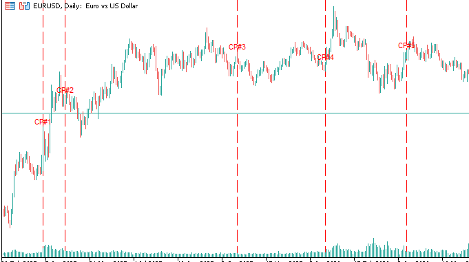
DrawOnChart() draws a dashed vertical line and a small label at each change point. It draws only when the chart shows the same symbol and timeframe that were analyzed, removes the objects of any earlier run first, and only reads results that are already final, so drawing never affects detection.
The optional sensitivity scan re-runs detection while varying one setting at a time, using the automatic penalty (InpPenalty is ignored): the penalty multiplied by 0.5, 1, 2 and 3, the minimum segment length set to 5, 10 and 20, and the lookback set to 0.8, 1.0 and 1.2 times InpLookback. It prints one line per run with the penalty used and the number and dates of the change points. A change point that keeps appearing near the same date is robust to these choices, and one that appears in only a few is borderline.
The script has seven inputs: InpSymbol, InpTimeframe, InpLookback, InpPenalty, InpMinSegmentLength, InpDrawOnChart and InpRunSensitivity. OnStart() is thin:
   CChangePointDetector detector;

   if(!detector.Run(symbol,
                    InpTimeframe,
                    InpLookback,
                    InpPenalty,
                    InpMinSegmentLength))
     {
      Print("Change Point Detection failed - check inputs, symbol/history availability.");
      return;
     }

   detector.PrintResults();

   if(InpDrawOnChart)
      detector.DrawOnChart();

   if(InpRunSensitivity)
      RunSensitivityScan(symbol);
The class can also be used from an Expert Advisor, but that does not turn its output into a validated real-time signal. It only means the same retrospective analysis can be re-run periodically.
Reading the Output
Here is the script run on EURUSD, Daily timeframe, with the default 500-bar lookback, the automatic penalty and InpMinSegmentLength = 10. It requests 500 closed bars and fetches 501 closed prices internally, so Total observations is 500. This is a single run on a single symbol, shown to illustrate how to read the output. It is not evidence that the method works across markets, periods or regimes.
The example covers 500 daily returns dated from 2024.11.01 to 2026.10.06, using the historical EURUSD data available in the terminal at the time of the run. Results may differ when using price histories from other servers or revised historical data.
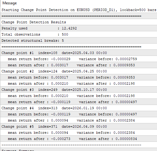
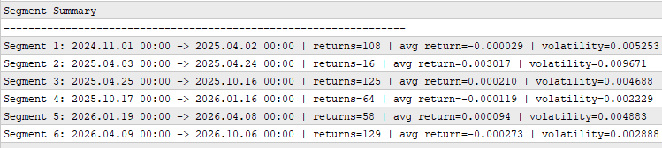
With n = 500 the automatic penalty is 2·ln(500) = 12.4292, exactly what is printed. Five change points produce six segments:
| Segment | Period (first → last return) | Returns | Avg return | Volatility |
|---|---|---|---|---|
| 1 | 2024.11.01 → 2025.04.02 | 108 | -0.000029 | 0.005253 |
| 2 | 2025.04.03 → 2025.04.24 | 16 | 0.003017 | 0.009671 |
| 3 | 2025.04.25 → 2025.10.16 | 125 | 0.000210 | 0.004688 |
| 4 | 2025.10.17 → 2026.01.16 | 64 | -0.000119 | 0.002229 |
| 5 | 2026.01.19 → 2026.04.08 | 58 | 0.000094 | 0.004883 |
| 6 | 2026.04.09 → 2026.10.06 | 129 | -0.000273 | 0.002888 |
Three conclusions follow.
There is one short burst of volatility. Segment 2 stands out. Its volatility is about 1.8 times that of the next-highest segment, and change points #1 and #2, only 16 returns apart, bracket it. The sturdier statement is that return volatility was sharply elevated for about three weeks. The return data alone cannot say whether the cause was a news release, a central bank event or a liquidity shock.
The changes in the mean are unconvincing. Every change point here is mainly a change in variance, by factors of 2.9 to 4.8 between neighboring segments. No segment's mean is more than about 1.25 standard errors from zero (Segment 2 at 1.25, Segment 6 at 1.07, the others at about 0.5 or less), so sign changes in the mean column, such as positive in Segment 3 and negative in Segment 4, should not be read as shifts in direction.
Short segments carry the most uncertainty. The relative error of a segment's volatility is roughly one over the square root of twice its number of returns. For Segment 2's 16 returns that is about 18%, with a standard error of the mean of about 0.0024. For Segment 6's 129 returns it is about 6% and 0.00025. A short segment can be a real detection, but its parameters are noisy.
One caution applies to all of this. These are the results of the penalized segmentation objective, and the variance estimates assume Gaussian returns, which real returns violate, as the simulation below shows. Because the still-forming bar is excluded and the penalty depends only on n, running the script again on the same history and inputs reproduces the same segmentation exactly.
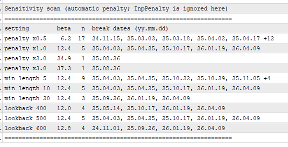
How stable is this segmentation?To see how much of this depends on the settings, I ran the sensitivity scan on the same EURUSD history. Dates are printed as yy.mm.dd, and a +N after the fifth date means that many more change points were found than are listed.
| Observation | Conclusion |
|---|---|
| The January and April 2026 boundaries (2026.01.19 and 2026.04.09) are preserved at minimum lengths 10 and 20 and at all three lookbacks | Relatively stable result |
| The autumn 2025 boundary moves: 2025.10.17 at the default, 2025.10.22 at minimum length 5, 2025.09.26 at minimum length 20 and lookback 600 | The period of change is determined better than the exact date |
| The short April 2025 episode disappears at lookback 600 and at both higher penalties (at lookback 400 the window starts too close to it, and at minimum length 20 it cannot appear) | A setting-sensitive result |
| Doubling the penalty gives a single change point on 2025.08.26, none of the five; tripling gives the same one | The penalty changes not only the number of boundaries but also their location |
Halving the penalty gives 17 change points, several about two weeks apart, which is the signature of the model chasing noise. The minimum length matters too, with 9, 5 and 3 change points at lengths 5, 10 and 20. Five change points in 500 returns is also close to the average the simulation below produces on fat-tailed data with no regime change at all, so the count by itself proves nothing. The scan separates the features that survive from the ones that do not: the early-2026 volatility swing is supported across most settings, the autumn 2025 calming is approximate, and the April 2025 spike is borderline.
How Often Does It Fire When Nothing Has Changed?
To see how the default settings behave, I ran the same algorithm (500 returns, automatic penalty, minimum segment length 10) on 150 simulated series of each of three kinds, none containing a deliberate regime change.
| Simulated returns | Runs with at least one change point | Average change points per run |
|---|---|---|
| Independent Gaussian (what the model assumes) | 14% | 0.2 |
| Independent Student-t, 3 degrees of freedom (fat tails) | 97% | 5.2 |
| GARCH(1,1) (volatility clustering) | 93% | 2.8 |
The Gaussian series used a standard deviation of 0.006, the Student-t series 3 degrees of freedom and a scale of 0.004, and the GARCH series ω = 2·10⁻⁷, α = 0.08, β = 0.90.
These results are illustrative Monte Carlo estimates based on 150 simulated series per model. They demonstrate the sensitivity of the default settings to distributional assumptions and should not be interpreted as universal or precisely calibrated false-alarm rates.
On data that matches the model's assumptions, the false-alarm rate is modest though not negligible. On fat-tailed data the detector fires almost every time, because a handful of extreme returns look to a Gaussian cost like a change in variance. On GARCH data, the segments describe volatility clustering rather than structural events. Real return series have both features, and nothing in a single run can tell the two apart, so detected change points are candidates to be checked against the sensitivity scan, not established events.
Conclusion
We built a complete Change Point Detector in MQL5: a Gaussian mean/variance segment cost, a penalized dynamic programming objective, and PELT pruning with deferred removal, organized into four reusable classes. The solver finds the exact optimum of the floored Gaussian objective. It prunes only when a checkable condition guarantees the pruning inequality for the floored cost, and otherwise runs the full recursion, so the result is exact either way. The output is a dated segmentation of a return history, useful as a basis for regime-conditioned testing of a strategy, for studying whether position-sizing rules should depend on volatility regimes, or simply as a record of when the modeled volatility of an instrument changed.
The main limitations are the ones stated at the start. The method is retrospective and cannot report change points in the most recent bars. It is repeatable but not assumption-free: on EURUSD, doubling the penalty replaces the five change points with a single, different one. The Gaussian cost does not capture heavy tails, volatility clustering or serial correlation, and the simulation shows how readily the default settings find change points in fat-tailed data. The implementation's explicit checks make it reject bad input and invalid states, but they do not make the model statistically correct.
Natural directions for development include regime-conditioned strategy validation, rolling or online detection for near-real-time alerts, cost functions built for heavy tails or GARCH-style variance (checked against the pruning condition), and Bayesian Change Point Detection, which would replace the fixed penalty with a probabilistic treatment of how likely a break is at each point.
Appendix A: Test Setup for the Pruning Checks
The checks were run with the attached script pelt_pruning_test.py, a Python port of the cost function and the recursion in ChangePointDetector.mq5. The main test uses a master seed (20261109); the efficiency check and the stress test use seeds derived from it (+1 and +2), and the minimum-length demonstration uses seeds 1 to 5, so the same seeds reproduce the same series and results.
Objective and variants. The objective is the floored Gaussian cost, C(s, e) = n·ln(max(var, ε)) with ε = 10⁻⁸ × var_all, and F(0) = −β. The reference is a brute-force dynamic program that tries every admissible τ and does no pruning. Three pruned variants are compared with it: immediate removal, deferred removal, and deferred removal guarded by the window check (smallest minSegLen-window variance at least 2ε), which is the variant the MQL5 script implements.
Matching criterion. A variant matches the brute-force result when the lists of change point indices are identical and the total objective F(n) agrees within 10⁻⁹ relative (10⁻⁷ absolute) tolerance.
Main test. 2,400 series, 400 of each of six types, generated through closing prices rounded to 5 decimal places (3 for the coarse-grid type): independent Gaussian returns (standard deviation 0.006); Student-t returns with 3 degrees of freedom (scale 0.004); GARCH(1,1) (ω = 2·10⁻⁷, α = 0.08, β = 0.90); random regime changes (segments of 10 to 60 returns, with random mean and volatility); Gaussian returns with one to three runs of identical closes; and small moves on a coarse price grid. Each series has 40 to 200 returns, a minimum segment length from 2 to 15, and a penalty of 0.5, 1 or 2 times 2·ln(n).
Floor-binding stress test. 29,814 series of 20 to 70 returns built from flat runs, tiny noise and ordinary noise, with minimum segment lengths from 2 to 6, so that the variance floor binds often.
Efficiency and minimum-length checks. The cost evaluation counts come from one 500-return regime-change series with a minimum length of 10 and the automatic penalty. The Python port evaluates each candidate cost once per endpoint, whereas the MQL5 listing recomputes it in the candidate-set pass, so evaluation counts taken from the MQL5 code are higher than those reported here. The minimum-length demonstration uses five 500-return Gaussian series with the automatic penalty.
Results. Immediate pruning differed from brute force on 74 of the 2,400 series. Deferred pruning, guarded or not, matched on all 2,400. The guard switched pruning off on 532 of them. In the stress test, deferred pruning without the guard differed on 30 of 29,814 series and the guarded version on none. These results come from the Python port, not from the MQL5 file itself.
Attached files:
| File | Type | Short description |
|---|---|---|
| ChangePointDetector.mq5 | MQL5 script (source code) | The change point detector. It prepares log returns, computes the floored Gaussian segment cost, runs PELT with deferred pruning, prints the segments, can draw them on the chart and can run the sensitivity scan. |
| pelt_pruning_test.py | Python 3 script | A test that compares the pruned PELT variants with a brute-force partitioner on simulated series, with a fixed seed. It also runs a floor-binding stress test, an efficiency check and a minimum-length demonstration. Run it with python pelt_pruning_test.py |
Warning: All rights to these materials are reserved by MetaQuotes Ltd. Copying or reprinting of these materials in whole or in part is prohibited.
This article was written by a user of the site and reflects their personal views. MetaQuotes Ltd is not responsible for the accuracy of the information presented, nor for any consequences resulting from the use of the solutions, strategies or recommendations described.