Testing Random Walk vs Mean Reversion in MQL5: Implementing the Lo-MacKinlay Variance Ratio Test

1. Introduction

Most trading strategies rely on some assumption about price behavior. Mean-reversion strategies expect prices to return to a reference level. Breakout strategies bet on continuation after a range break. Both can work—until market conditions shift. When that happens, a strategy optimized for one regime often fails in another.

A price chart alone can't formally validate these assumptions. Indicators like RSI or Bollinger Bands describe recent price behavior, but they don't test whether returns actually exhibit the serial dependence a strategy expects. An oversold RSI reading doesn't guarantee mean-reversion—it just shows where price sits relative to recent history. So let's step back and ask a more fundamental question: are return increments consistent with the variance-scaling implication of a random-walk or martingale-difference null, or is there measurable dependence across different holding horizons?

Here, we'll implement the Lo-MacKinlay Variance Ratio Test (1988) in MQL5. The test checks whether the variance of k-period returns scales the way a random-walk or martingale-difference null implies it should—specifically, whether the variance of k-period returns grows proportionally with k.

It's worth being precise about scope here: rejecting the null is evidence against that specific variance-scaling property. It is not a general proof or disproof of "the market is or isn't a random walk" in every sense—structural breaks, microstructure noise, and general nonlinear dependence are not directly captured by a VR statistic. This article uses two nulls. The classical homoskedastic statistic tests compatibility with iid increments (a strict random walk with constant variance). The heteroskedasticity-robust statistic tests a weaker null: uncorrelated increments with time-varying variance (a martingale-difference sequence). The robust version is best read as a test of the variance-scaling implication under a null of no linear serial dependence in returns, allowing for heteroskedasticity.

VR(k) ≈ 1 is consistent with the null. Below 1 suggests that negative autocorrelation outweighs positive autocorrelation across the horizon; above 1 suggests the reverse. But sampling variation can push VR away from 1 even under the null. That's why we need the Z-statistic, which scales the deviation by its estimated sampling variability. It's a useful guide only under conditions: the asymptotic normal approximation has to hold reasonably well at the sample size used, the variance term φ has to be normalized correctly (Section 3.4 spells this out), and the lags and window have to be fixed before looking at the results.

One more caveat worth flagging up front: on very short timeframes (M1, M5, and similar), a VR below 1 is often driven by market microstructure effects — bid-ask bounce, non-synchronous trading, discrete tick sizes — rather than any economically meaningful reversal in price. The test doesn't distinguish between the two; it only measures whether variance scales as the null predicts. That distinction matters more the shorter the bar interval gets.

We'll implement this as an on-demand diagnostic tool rather than a continuous indicator. The code is split into two files:

• VarianceRatio.mqh – Contains the statistical engine (zero-dependency CVarianceRatio class) with both the classical homoskedastic test and the heteroskedasticity-robust version.
• VarianceRatioScript.mq5 – Handles data retrieval, runs the test across multiple horizons, and logs the results.

This separation is deliberate. The engine doesn't care about charts, trading decisions, or display—it just processes price data. That makes CVarianceRatio reusable: call it from a script for diagnostics, or drop it directly into an EA when you need a statistical gate.

By the end, you'll have a practical diagnostic that tests multiple horizons and identifies statistically significant departures from random-walk-implied variance scaling at the selected horizons. Producing the numbers is the easy part. Reading them correctly is the point. A VR below 1 isn't proof of mean-reversion, just as a VR above 1 isn't proof of a trend. Statistical significance is what matters here, though even that needs careful reading once you're scanning several horizons at once.

2. The Variance Ratio Hypothesis

2.1 Theoretical intuition

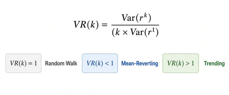
The Variance Ratio test starts with a simple property of a random walk. Under the random-walk null, the variance of a k-period return should scale proportionally with k. For a holding period of k periods, the expected relationship is:

$$\text{<b>Var</b>}<b>(</b>{\mathrm{<b>r</b>}}_{\mathrm{<b>t</b>}}^{\mathrm{<b>k</b>}}<b>)</b><b>=</b>\mathrm{<b>k</b>}<b>\cdot </b>\text{<b>Var</b>}<b>(</b>{\mathrm{<b>r</b>}}_{\mathrm{<b>t</b>}}^{\mathrm{<b>1</b>}}<b>)</b>$$

In other words, if the holding horizon becomes twice as long, the variance should also become twice as large under the random-walk assumption. That's the core idea. We're not predicting the next price—we're testing whether uncertainty accumulates the way a random walk would predict. If variance grows slower than expected, returns are offsetting each other more than under independence. If it grows faster, returns are moving together more than the random-walk model predicts.

2.2 The VR(k) metric

The Variance Ratio turns that idea into a measurable quantity. For a given horizon k, we compare the observed variance of the k-period returns with the variance that would be expected from k one-period returns under the random-walk assumption:

$$\mathrm{<b>V</b>}\mathrm{<b>R</b>}<b>(</b>\mathrm{<b>k</b>}<b>)</b><b>=</b>\frac{\text{<b>Var</b>}<b>(</b>{\mathrm{<b>r</b>}}_{\mathrm{<b>t</b>}}^{\mathrm{<b>k</b>}}<b>)</b>}{\mathrm{<b>k</b>}<b>\cdot </b>\text{<b>Var</b>}<b>(</b>{\mathrm{<b>r</b>}}_{\mathrm{<b>t</b>}}^{\mathrm{<b>1</b>}}<b>)</b>}$$

The denominator represents the variance we would expect if the one-period returns simply accumulated without serial dependence. The numerator represents what we actually observe over the longer horizon.

In practice, the sample estimator used in this implementation is built from overlapping k-period returns with the Lo–MacKinlay finite-sample adjustment in the denominator, rather than a naive ratio of two independently computed sample variances. Section 3.4 shows this estimator in full — the formula above is the theoretical definition; the code implements its finite-sample, overlapping-return counterpart.

VR(k) gives us three possible outcomes:

VR(k) value	Direction	Meaning
= 1.0	None	Behavior consistent with random-walk scaling
< 1.0	Negative serial dependence	Variance grows more slowly than random-walk scaling
> 1.0	Positive serial dependence	Variance grows faster than random-walk scaling

VR < 1 means the weighted sum of return autocorrelations up to lag k−1 is negative. To a first approximation, VR(k) − 1 ≈ 2·Σ (1 − j/k)·ρ(j) for j = 1 to k−1, where ρ(j) is the lag-j autocorrelation of one-period returns, and the weights taper off as j approaches k. That describes the net effect, not every lag: short-lag negative autocorrelation can outweigh a positive one further out, and VR alone can't tell you which lags are doing the work. A net-negative sum is consistent with one form of short-horizon reversal behavior relevant to some mean-reversion strategies — but it is not the same claim as classical mean reversion of price toward a fundamental or reference level, and it doesn't by itself prove any mean-reversion effect is tradable.

Plenty of mean-reversion strategies aren't built on linear autocorrelation in returns at all — reversion in a spread, deviation from a cointegrating relationship, or intraday inventory effects, for instance — so a VR result speaks only to this one specific form of dependence. The strength and persistence of this effect matter separately.

VR > 1 means the same weighted sum is positive, so positive autocorrelation outweighs negative across the horizon, again as a net result rather than a lag-by-lag statement. But VR alone isn't a statistical conclusion—sampling variation can push it away from 1. That's why we calculate the Z-statistic: it scales the departure by its estimated sampling variation so we can judge whether it is large relative to that noise.

2.3 Homoskedastic vs heteroskedasticity-robust statistics

The classical version assumes constant variance—convenient, but rarely realistic for financial returns. Volatility clusters. Quiet periods and turbulent periods alternate, and the uncertainty associated with returns changes over the sample.

Lo and MacKinlay's solution is a heteroskedasticity-consistent estimator, φ*(k), which incorporates lag-specific δ(j) terms to correct the estimate of VR's sampling variance for time-varying volatility. The exact formula, and the scaling convention this article uses, are given in Section 3.4, Stage 4, alongside the code that implements it, so the mapping between the two can be checked directly.

The robust Z*(k) adjusts for changing volatility. Ignoring heteroskedasticity distorts the estimated uncertainty of the VR statistic, which can change whether a result looks significant. That's why the robust version is generally the better choice for financial returns, where volatility rarely stays constant. Our implementation calculates both versions, the classical one as a reference, and the robust one as the primary diagnostic for financial data.

3. Code Architecture: The Engine (VarianceRatio.mqh)

The CVarianceRatio class separates the statistical logic from the chart-facing code, making it reusable across scripts, indicators, and EAs.

3.1 Class surface

The public interface is deliberately small:

//+--------------------------------------------------------------------+
//| CVarianceRatio                                                     |
//|                                                                    |
//| Implements the Lo-MacKinlay Variance Ratio test using overlapping  |
//| k-period returns, with both the classical homoskedastic asymptotic |
//| variance and the heteroskedasticity-consistent asymptotic variance.|
//| Scope of the null hypothesis is discussed in the accompanying      |
//| article.                                                           |
//+--------------------------------------------------------------------+
class CVarianceRatio
  {
private:
   int               m_window_size;     // Rolling sample size (number of 1-period log returns used)
   int               m_min_window;      // Minimum viable window (safety floor)

   //--- internal return buffer
   double            m_returns[];       // 1-period log returns buffer

   //--- helpers
   bool              BuildLogReturns(const double &prices[], const int count, double &out_returns[]);
   bool              ComputeVarianceRatioCore(const double &returns[], const int n, const int k,
         double &vr, double &z_homo, double &z_hetero);
   double            SafeDiv(const double numerator, const double denominator, const double fallback = 0.0);

public:
                     CVarianceRatio(void);
                    ~CVarianceRatio(void);

   //--- configuration
   void              SetWindowSize(int window);
   int               GetWindowSize(void) const { return m_window_size; }

   //--- core API
   bool              Calculate(const double &prices[], const int k,
                               double &vr, double &z_homo, double &z_hetero);

   //--- ok_out[i] flags success/failure per lag (see article, Section 3.5)
   bool              CalculateMultiLag(const double &prices[], const int &lags[],
                                       double &vr_out[], double &z_out[], bool &ok_out[]);
  };

The class exposes two main methods:

• Calculate() – Runs the test for a single lag, returning VR, homo Z, and robust Z.
• CalculateMultiLag() – Runs the test across multiple lags in one call, and also returns an explicit ok_out[] status array (see Section 3.5).

SetWindowSize() enforces a minimum of 20 returns—an implementation safeguard, not a formal requirement of the Lo-MacKinlay test. It's worth being clear about what that number means: 20 is not a claim that 20 returns are sufficient for a reliable test. The Z-statistics here rely on asymptotic approximations that can behave poorly at small sample sizes, and 20 is simply a floor against obviously degenerate input, not a minimum sample size the test has been shown to work well at. Sample size should always be considered when interpreting output, and in practice the 200-return window used throughout this article is doing the real work, not the 20-return floor. Because the engine may clamp the value you ask for, callers should read the effective window back with GetWindowSize() rather than assuming their request was accepted; the script and the EA below do exactly that.

ComputeVarianceRatioCore() also explicitly rejects k < 2 or k >= n (the number of returns in the window) before any statistic is computed, rather than letting bad values reach the arithmetic. This keeps the failure mode explicit: calling Calculate() with, say, k = 1 from an EA fails loudly with a printed reason instead of silently returning a degenerate or meaningless statistic. The actual work happens in ComputeVarianceRatioCore(), but before that, the engine converts prices to returns.

3.2 Building log returns

The test operates on returns rather than raw prices. The conversion is handled by BuildLogReturns():

//+--------------------------------------------------------------------+
//| BuildLogReturns                                                    |
//| Converts a price series (oldest -> newest, non-timeseries order)   |
//| into 1-period log returns. Validates positivity of prices to avoid |
//| NaN from log(<=0).                                                 |
//+--------------------------------------------------------------------+
bool CVarianceRatio::BuildLogReturns(const double &prices[], const int count, double &out_returns[])
  {
   if(count < 2)
      return false;

   ArrayResize(out_returns, count - 1);

   for(int i = 1; i < count; i++)
     {
      double p0 = prices[i - 1];
      double p1 = prices[i];

      if(p0 <= 0.0 || p1 <= 0.0)
        {
         Print("CVarianceRatio::BuildLogReturns: non-positive price encountered, aborting calculation.");
         return false;
        }

      out_returns[i - 1] = MathLog(p1 / p0);
     }

   return true;
  }

With N prices, there are N-1 one-period returns. Each return is calculated as:

$${\mathrm{<b>r</b>}}_{\mathrm{<b>t</b>}}<b>=</b>\mathrm{<b>ln</b>}<b></b><b>(</b>\frac{{\mathrm{<b>P</b>}}_{\mathrm{<b>t</b>}}}{{\mathrm{<b>P</b>}}_{\mathrm{<b>t</b>}<b>-</b>\mathrm{<b>1</b>}}}<b>)</b>$$

The chronological ordering is preserved because the test is built on how returns at different points in time relate to one another, and because Calculate() treats the end of the array as the most recent data. If prices[] arrived newest→oldest, this function would still run without error, but each r_t would be the negative of the return it should represent, in reversed time order. Section 4.2 covers what that does and doesn't break.

The positivity check is also important. A non-positive price would make the logarithm invalid, potentially introducing an invalid value into the return series and contaminating the subsequent calculations. The implementation therefore stops rather than allowing a bad observation to propagate through the test.

3.3 Orchestrating a single calculation (Calculate())

BuildLogReturns() converts prices into returns, but something has to decide how many prices actually go into that conversion. That's the job of Calculate() — the public entry point that ties the return-building step to the core statistics:

//+--------------------------------------------------------------------+
//| Calculate                                                          |
//| Public entry point for a single lag k. prices[] must be in         |
//| chronological (oldest -> newest) order. Uses the most recent       |
//| m_window_size+1 prices (needs +1 to produce m_window_size returns).|
//+--------------------------------------------------------------------+
bool CVarianceRatio::Calculate(const double &prices[], const int k,
                               double &vr, double &z_homo, double &z_hetero)
  {
   vr = 1.0;
   z_homo = 0.0;
   z_hetero = 0.0;

   int total = ArraySize(prices);
   int needed_prices = m_window_size + 1;

   if(total < needed_prices)
     {
      PrintFormat("CVarianceRatio::Calculate: not enough price data (have %d, need %d).",
                  total, needed_prices);
      return false;
     }

//--- Use only the trailing window (most recent needed_prices elements)
   double window_prices[];
   ArrayResize(window_prices, needed_prices);
   int start = total - needed_prices;
   for(int i = 0; i < needed_prices; i++)
      window_prices[i] = prices[start + i];

   if(!BuildLogReturns(window_prices, needed_prices, m_returns))
      return false;

   int n = ArraySize(m_returns);
   return ComputeVarianceRatioCore(m_returns, n, k, vr, z_homo, z_hetero);
  }

Three things are worth pointing out here.

First, the function always works from the trailing slice of the price array — the most recent m_window_size + 1 prices, regardless of how many prices were actually passed in. The "+1" is because BuildLogReturns() turns N prices into N−1 returns, so this is exactly the number of prices needed to produce a return series of length m_window_size.

Second, the window is independent of the lag k. Calculate() doesn't adjust the slice size based on the requested horizon. The same window is reused whether k is 2 or 20. Any lag-specific sizing requirement is instead handled downstream, inside ComputeVarianceRatioCore()'s lag and window-length guards.

Third, defaulting vr = 1.0 before any validation is a deliberate choice: the outputs are initialized to neutral values before validation so that a failed calculation does not leave stale results from a previous call.

3.4 Computing the Variance Ratio

Once the return series has been built, ComputeVarianceRatioCore() performs the main calculation. The implementation can be viewed as four stages, preceded by two validity guards.

Guards: lag and window length

//--- Explicit lag validity check (see article, Section 3.4).
   if(k < 2 || k >= n)
     {
      PrintFormat("CVarianceRatio::ComputeVarianceRatioCore: invalid lag k=%d for n=%d returns (need 2 <= k < n).",
                  k, n);
      return false;
     }

//--- Window-length safeguard: require at least 4*k returns (and never
//--- fewer than the global floor). This is an implementation choice
//--- against very sparse samples, not a formal requirement of the
//--- Lo-MacKinlay test itself.
   if(n < k * 4 || n < m_min_window)
     {
      PrintFormat("CVarianceRatio::ComputeVarianceRatioCore: insufficient samples (have %d, need >= %d) for k=%d.",
                  n, MathMax(k * 4, m_min_window), k);
      return false;
     }

k = 1 is a degenerate case for this test: the homoskedastic asymptotic variance phi_homo collapses to 0, and the loop that builds the robust variance never executes (it runs over j = 1..k-1, which is empty when k = 1). At the other end, for k >= n the problem isn't simply that there's "less overlap" — the overlapping-return estimator and its finite-sample denominator m degenerate outright: at k = n there is exactly one k-period cumulative return to work with, and the asymptotic variance formulas built on n observations of overlapping windows stop being meaningful in that finite sample. Both cases are rejected explicitly rather than being allowed to produce a nonsensical or zero statistic.

The second guard requires the window to hold at least four times k returns (and never fewer than the 20-return floor). Like the floor, this is an implementation safeguard against very sparse samples, not part of the Lo-MacKinlay test. With the default 200-return window it only matters for lags above 50.

Stage 1: One-period variance

Calculate mean and sample variance:

//--- mean of 1-period returns
   double sum = 0.0;
   for(int t = 0; t < n; t++)
      sum += returns[t];
   double mu = sum / n;

//--- unbiased 1-period variance (sigma_a^2), divisor (n-1)
   double ss1 = 0.0;
   for(int t = 0; t < n; t++)
     {
      double d = returns[t] - mu;
      ss1 += d * d;
     }
   double var1 = SafeDiv(ss1, (double)(n - 1), 0.0);
   if(var1 <= 0.0)
     {
      Print("CVarianceRatio::ComputeVarianceRatioCore: degenerate 1-period variance (flat price series?).");
      return false;
     }

The variance uses n - 1 in the denominator, giving the usual unbiased sample variance. If the resulting variance is zero, the calculation is stopped because a constant return series cannot provide a meaningful variance ratio. The accumulated squared deviations ss1 are retained because they are also needed later when constructing the heteroskedasticity-consistent statistic.

Stage 2: Overlapping k-period variance

For the longer-horizon variance, we use all overlapping windows:

//--- k-period overlapping variance (sigma_c^2)
//--- m is the standard Lo-MacKinlay bias-adjustment divisor, derived for
//--- exactly (n - k + 1) overlapping k-period windows.
//--- For 2 <= k < n every factor is positive, so m > 0 always holds once
//--- the lag guard above has passed; the check below is purely defensive.
   double m = k * (n - k + 1) * (1.0 - (double)k / (double)n);
   if(m <= 0.0)
     {
      Print("CVarianceRatio::ComputeVarianceRatioCore: degenerate overlapping-sample adjustment.");
      return false;
     }

//--- t = k-1 .. n-1 (zero-based) -> (n - k + 1) overlapping windows total,
//--- with the first window (t = k-1) covering indices 0..k-1.
   double sumk = 0.0;
   for(int t = k - 1; t < n; t++)
     {
      double cum = 0.0;
      for(int i = t - k + 1; i <= t; i++)
         cum += returns[i];
      double dk = cum - k * mu;
      sumk += dk * dk;
     }
   double vark = SafeDiv(sumk, m, 0.0);

//--- fallback is 0.0 (not 1.0) so a future refactor cannot make a failed
//--- division silently resolve to "VR = 1".
   vr = SafeDiv(vark, var1, 0.0);

Log returns are additive, so summing k consecutive returns gives the k-period return. Overlapping windows let every observation contribute to the estimate. That's part of the test's design, not a shortcut taken in the code. The divisor m applies the Lo-MacKinlay overlapping-sample adjustment. For any k that passes the lag guard (2 ≤ k < n), every factor in m is positive, so m is strictly positive and the m <= 0 check can't actually fire. It stays as a defensive check in case the guard is ever loosened. In practice the binding constraint is the second guard described above, which requires at least four times k returns. Finally, the longer-horizon variance is divided by the one-period variance to obtain VR(k).

Two things worth being precise about here. First, n throughout this function is the number of one-period returns in the window, not the number of prices — Calculate() converts m_window_size + 1 prices into m_window_size returns before this function ever sees them, so n and m_window_size are the same quantity by the time this code runs. Second, dk = cum - k * mu demeans each k-period cumulative return using mu, the overall one-period return mean computed in Stage 1 — not a separately computed mean of the k-period return series itself.

That's not a simplification; it's the exact form the Lo–MacKinlay overlapping-return estimator calls for, and changing it to demean against a k-period series' own mean would silently break the formula's correspondence to the paper. The vr = SafeDiv(vark, var1, 0.0) fallback is dead code in practice — var1 <= 0.0 already returns false earlier in this function — but it's written as 0.0 rather than 1.0 specifically so that if this function is ever refactored and that earlier guard is weakened, an unreachable-in-theory division doesn't quietly resolve to "VR = 1" by default.

Stage 3: Classical homoskedastic statistic

The classical Z-statistic uses the asymptotic variance derived under the homoskedastic assumption:

//--- Homoskedastic asymptotic variance phi(k), the variance of VR(k) itself
   double phi_homo = (2.0 * (2.0 * k - 1.0) * (k - 1.0)) / (3.0 * k * n);
   z_homo = (phi_homo > 0.0) ? SafeDiv(vr - 1.0, MathSqrt(phi_homo), 0.0) : 0.0;

The calculation follows the usual structure:

Z(k) = (VR(k)-1)/√φ(k)

The purpose of this statistic is to scale the deviation of the variance ratio from its random-walk benchmark by its estimated sampling variability. Under the null hypothesis, VR(k) is expected to be close to 1. The Z-statistic tells us how far the observed value is from that benchmark relative to the estimated variability of the statistic, with the usual proviso that the normal approximation only holds asymptotically. The homoskedastic version is retained because it provides a useful reference, but financial returns often violate its constant-variance assumption.

Stage 4: Heteroskedasticity-consistent statistic

The robust statistic replaces the simple asymptotic variance with an estimator of VR's variance that remains valid when volatility changes over time. Written out in full, the estimator is:

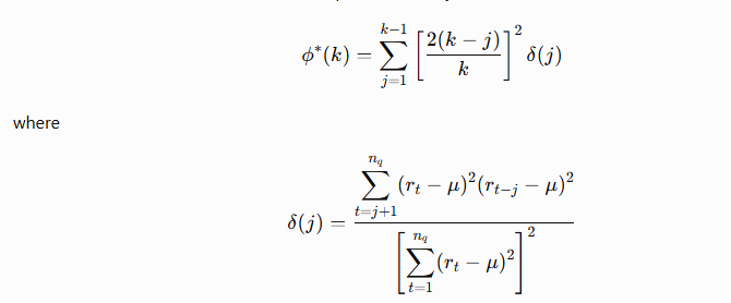
Mapping to the code: ss1 = Σ(r_t − μ)² is the raw sum of squared centered returns. Rather than dividing by ss1² directly, the code rescales each squared deviation by the mean squared deviation, w_t = (r_t − μ)² / (ss1/n). Since Σw_t = n, δ(j) = Σ w_t·w_{t−j} / n², which is algebraically identical to the numerator-over-ss1² form in the formula above. phi_hetero then accumulates weight² · δ(j) across j = 1..k−1, matching the summation in φ*(k) term for term. The rescaling is deliberate: return variances are small numbers, so ss1² can fall near or below any fixed absolute threshold even for a perfectly valid series. Working with w_t keeps every intermediate quantity of order 1 and avoids an arbitrary cutoff. The formula block above is the reference. If you check the code against Lo & MacKinlay (1988) directly, keep the scaling note that follows in mind.

A note on scaling, because it directly affects Z*(k). In the standard presentation, θ(k) and θ*(k) are the asymptotic variances of √n·(VR(k) − 1), and δ(j) carries a factor of n in its numerator. This article works with the variance of VR(k) itself, which is smaller by a factor of n, so φ(k) = θ(k)/n in Stage 3 and φ*(k) = θ*(k)/n here. That's why the code computes δ(j) without the n multiplier: the factor in the numerator and the 1/n conversion cancel. The scaling is easy to check. If returns are homoskedastic, each cross-product sum is roughly nσ⁴ and ss1² is roughly n²σ⁴, so δ(j) comes out near 1/n. The squared weights then sum to 2(2k−1)(k−1)/(3k), and φ*(k) collapses to the φ(k) from Stage 3, as it should. Keeping the multiplier without dividing by n later would inflate φ*(k) about n-fold and shrink every robust Z by roughly √n, a factor near 14 at a 200-return window. Since Z*(k) is compared against standard normal critical values, this normalization is what makes that comparison valid.

//--- Heteroskedastic-robust asymptotic variance phi*(k)
//--- Scale-invariant form: each squared deviation is divided by the mean
//--- squared deviation (ss1/n), w_t = (r_t - mu)^2 / (ss1/n). Then
//--- sum(w_t) = n and delta_j = sum_{t=j}^{n-1} w_t * w_{t-j} / n^2,
//--- which equals num / ss1^2 exactly but needs no absolute threshold
//--- on ss1^2 (small valid return variances can fall far below any
//--- fixed epsilon). delta_j is already on the scale of phi(k) (divided
//--- by n), so phi_hetero is the variance of VR(k) itself.
   double scale = ss1 / (double)n;   // > 0 here because var1 > 0
   double w[];
   ArrayResize(w, n);
   for(int t = 0; t < n; t++)
     {
      double d = returns[t] - mu;
      w[t] = (d * d) / scale;
     }

   double n_sq = (double)n * (double)n;
   double phi_hetero = 0.0;

   for(int j = 1; j <= k - 1; j++)
     {
      double num = 0.0;
      for(int t = j; t < n; t++) // t = j .. n-1 (zero-based), matches sum_{t=j+1}^{n} in 1-based math
         num += w[t] * w[t - j];

      double delta_j = num / n_sq;
      double weight  = 2.0 * (k - j) / (double)k;
      phi_hetero += weight * weight * delta_j;
     }

//--- If phi*(k) cannot be formed, report failure instead of returning a
//--- neutral z_hetero = 0.0 that looks like a genuine "no departure" result.
   if(!MathIsValidNumber(phi_hetero) || phi_hetero <= 0.0)
     {
      PrintFormat("CVarianceRatio::Calculate: robust variance phi*(k) is not positive/finite for k=%d.", k);
      return false;
     }

   z_hetero = (vr - 1.0) / MathSqrt(phi_hetero);

   return true;
  }

The key idea is that the variance of VR(k) is estimated using squared, centered returns. Each δ(j) is built from products of squared deviations at lag j, and the weights combine them into φ*(k), an estimate of VR's sampling variance that stays valid when volatility changes. To be clear about what this is: it doesn't test for dependence in the magnitude of returns as a separate hypothesis. It only changes the yardstick against which VR(k) − 1 is measured. If φ*(k) comes out non-finite or non-positive, the engine reports failure ( return false ) rather than returning z_hetero = 0.0, because a zero would be indistinguishable from a genuine “no departure” result.

The resulting z_hetero provides the statistic used for the robust interpretation of the test. Depending on how volatility clusters in the sample, the robust variance can come out larger or smaller than the classical one, which is why Z*(k) can end up above or below Z(k), as Section 5.2 shows.

3.5 Testing Multiple Horizons

For convenience, CalculateMultiLag() tests several holding periods in one call:

//+--------------------------------------------------------------------+
//| CalculateMultiLag                                                  |
//| Runs the calculation for several lags; ok_out[] flags per-lag      |
//| success (see article, Section 3.5).                                |
//+--------------------------------------------------------------------+
bool CVarianceRatio::CalculateMultiLag(const double &prices[], const int &lags[],
                                       double &vr_out[], double &z_out[], bool &ok_out[])
  {
   int lag_count = ArraySize(lags);
   if(lag_count <= 0)
     {
      Print("CVarianceRatio::CalculateMultiLag: empty lags array.");
      return false;
     }

   ArrayResize(vr_out, lag_count);
   ArrayResize(z_out, lag_count);
   ArrayResize(ok_out, lag_count);

   bool any_ok = false;

   for(int i = 0; i < lag_count; i++)
     {
      double vr, z_homo, z_hetero;
      bool ok = Calculate(prices, lags[i], vr, z_homo, z_hetero);

      ok_out[i] = ok;

      if(!ok)
        {
         //--- EMPTY_VALUE kept for display only; ok_out[i] is authoritative.
         vr_out[i] = EMPTY_VALUE;
         z_out[i]  = EMPTY_VALUE;
         continue;
        }

      vr_out[i] = vr;
      z_out[i]  = z_hetero;
      any_ok = true;
     }

   return any_ok;
  }

Each requested lag is passed through the same calculation pipeline. The output contains the variance ratio and the heteroskedasticity-consistent Z-statistic for each horizon. Failed lags are flagged through an explicit ok_out[] status array — in addition to still carrying EMPTY_VALUE in vr_out / z_out for convenience when printing — so callers never need to rely on exact floating-point comparison against EMPTY_VALUE to detect a failure. The method returns true if at least one lag was calculated successfully.

Worth being upfront about a tradeoff here: this implementation favors a simple API over raw efficiency. Each call to Calculate() re-slices the price window and rebuilds the entire log-return series from scratch, even though every lag in a multi-lag scan is working from the exact same underlying returns — only the core calculation past that point actually depends on k. For the handful of lags used in this article that cost is negligible. If this were extended to scan dozens of lags, or run on a tight loop, it would be worth building the return series once and calling ComputeVarianceRatioCore() directly for each lag instead.

4. The Diagnostic Script (VarianceRatioScript.mq5)

The engine now handles the statistics, so the script only needs to provide a practical interface around it. Its job is straightforward: collect the inputs, retrieve the required price history, run the test across the selected horizons, and present the results in a readable form.

Note that the script includes the engine as <Quantitative/VarianceRatio.mqh>, so save the header under MQL5/Include/Quantitative/. If you'd rather keep both files in one folder, change that line to #include "VarianceRatio.mqh".

4.1 Inputs and lag parsing

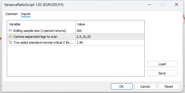
The script exposes three parameters:

#property script_show_inputs

#include <Quantitative/VarianceRatio.mqh>

//--- Inputs
input int    InpWindowSize = 200;         // Rolling sample size (1-period returns)
input string InpLags       = "2,5,10,20"; // Comma-separated lags to scan
input double InpCriticalZ  = 1.96;        // Two-sided standard-normal critical Z threshold

A script runs once when you drop it on a chart, unlike an indicator or EA, which keeps running. That's what makes this an on-demand diagnostic. #property script_show_inputs only tells the terminal to show the input dialog before that single run, so you can set the window, lags and threshold. The lag list is entered as a string because MQL5 input parameters do not support array inputs. The script parses the string into individual integers, trims the values, rejects lags below the engine's minimum of 2, and drops duplicates so the multiple-testing correction in Section 4.3 counts each horizon once. This keeps the input simple while still allowing several holding horizons to be tested from the same script.

4.2 Fetching prices in chronological order

The script then configures the engine and requests price history for the selected window:

//--- 2. Configure the engine, then fetch chronological price history.
//--- The engine may clamp the requested window, so its effective value is
//--- read back rather than assuming InpWindowSize was accepted.
//--- start_pos = 1 skips bar 0, which is still forming, so only fully
//--- closed bars enter the return series. Ordering is verified through
//--- each bar's .time field instead of being assumed.
   CVarianceRatio vrEngine;
   vrEngine.SetWindowSize(InpWindowSize);
   int effectiveWindow = vrEngine.GetWindowSize();
   int needed = effectiveWindow + 1; // window_size + 1 prices -> window_size returns

   MqlRates rates[];
   int copied = CopyRates(_Symbol, _Period, 1, needed + 10, rates);

   if(copied < needed)   // also catches copied == -1
     {
      PrintFormat("VarianceRatioScript: insufficient history on %s (%s) -- copied %d bars, need at least %d.",
                  _Symbol, EnumToString((ENUM_TIMEFRAMES)_Period), copied, needed);
      return;
     }

   bool alreadyChronological = (rates[0].time < rates[copied - 1].time);

   double closeArr[];
   ArrayResize(closeArr, copied);
   for(int i = 0; i < copied; i++)
      closeArr[i] = alreadyChronological ? rates[i].close : rates[copied - 1 - i].close;

This is easy to get wrong. CVarianceRatio expects prices[] in chronological order (oldest → newest). In MQL5, Copy*() ordering can vary with array settings and the copy function, so the script verifies ordering via the.time fields and reverses data if needed. Rather than asserting an order and hoping it holds, the code above sidesteps the question entirely: it reads each bar's own.time field from the returned MqlRates array and checks directly whether rates[0] is older or newer than rates[copied-1]. Whichever way the data actually came back, closeArr[] is then built explicitly into oldest → newest order from that observed fact, not from an assumption about it.

Skipping this step doesn't produce an error either; the script would still run and print numbers. The damage is subtler than a sign flip. Reversing a complete return series negates each return and mirrors the time order, but VR(k) and both Z-statistics come out the same, because they depend only on squared deviations, overlapping sums and lag-j products of squared returns, all of which are unchanged by the reversal. What breaks is which data gets tested. The engine keeps only the trailing window_size + 1 elements, so with newest→oldest data it would analyze the oldest bars in the buffer instead of the most recent ones. Here that's a shift of ten bars, but a caller passing a long history would be testing a window from the far past and reading it as current.

k does not change how much price data is required: the engine only ever consumes the trailing window_size + 1 prices regardless of the horizon being tested; k only affects how the overlap adjustment behaves inside the core calculation. The extra +10 above is just a small margin of additional bars. It is not needed by the calculation itself, since the engine keeps only the trailing slice.

Three details in that snippet are deliberate. The copy starts at position 1 because bar 0 is still forming, and its "close" is just the latest tick. The copied < needed check comes before any access to rates[0] or rates[copied - 1], since CopyRates() returns -1 on failure. And the script asks the engine for its effective window instead of using InpWindowSize directly: enter 10 and SetWindowSize() clamps it to 20, so the download has to cover 21 prices, not 11.

4.3 Multi-horizon run and strongest-signal detection

The script can evaluate all requested horizons through the engine's multi-lag interface:

//--- 3. Batch scan: CalculateMultiLag() returns the robust Z-score
//--- for each requested lag in a single call, with an explicit
//--- per-lag success flag (ok_batch) rather than relying on comparing
//--- doubles against EMPTY_VALUE.
   double vr_batch[], z_batch[];
   bool ok_batch[];
   bool batchOk = vrEngine.CalculateMultiLag(closeArr, lags, vr_batch, z_batch, ok_batch);

   int bestIdx = -1;
   double bestAbsZ = -1.0;
   int testedCount = 0;

   if(batchOk)
     {
      for(int i = 0; i < lagCount; i++)
        {
         if(!ok_batch[i])
            continue;

         testedCount++;

         double absZ = MathAbs(z_batch[i]);

         if(absZ > bestAbsZ)
           {
            bestAbsZ = absZ;
            bestIdx  = i;
           }
        }
     }

The batch calculation returns the robust Z-statistic for each horizon, along with an explicit success flag per lag. The script counts the lags that actually computed and compares their absolute values to find the largest observed absolute test statistic among the requested horizons. For the detailed output, the script also calls Calculate() for each valid lag so that the classical and robust statistics can be displayed side by side.

One qualification matters here: this largest-observed-statistic value isn't automatically a significant one, and "strongest signal" — the label used for it in the script's output below — is a convenient name for that quantity, not a claim about its statistical meaning. Each lag represents a separate hypothesis test, so scanning many horizons increases the chance of finding a large statistic simply through random variation. To make this concrete rather than just a caveat, the script also computes and prints a Bonferroni-adjusted critical Z-value. It takes the two-sided α implied by whatever critical Z you chose (0.05 at the default 1.96), divides it by the number of lags that actually computed, and converts the result back to a Z-threshold with the inverse standard normal CDF.

Deriving α from the input keeps the naive and adjusted thresholds on the same significance level, and counting only successful lags keeps the correction tied to the hypotheses actually tested. NormSInv() uses Acklam's rational approximation and NormCDF() a small Abramowitz–Stegun approximation; both are in the attached VarianceRatioScript.mq5 and aren't reproduced here.

//--- 3b. Bonferroni-adjusted threshold for multiple testing. alpha is
//--- derived from InpCriticalZ so the naive and adjusted thresholds refer
//--- to the same significance level, and only lags that actually
//--- computed are counted as tests.
   double alpha = 2.0 * (1.0 - NormCDF(InpCriticalZ));
   double bonferroniAlpha = (testedCount > 0) ? alpha / testedCount : alpha;
   double bonferroniZ = -NormSInv(bonferroniAlpha / 2.0); // two-sided

Bonferroni is on the conservative side; Holm's step-down procedure gives up less power if that matters more to you. Either beats not correcting at all — though it's worth adding one nuance here: Bonferroni does not require the tests to be independent for its family-wise error-rate bound to remain valid. The VR statistics at different horizons are built from overlapping windows of the same underlying data, and adjacent lags in particular can be strongly dependent on each other. That dependence can make the Bonferroni correction more conservative than it would be for genuinely independent tests.

The "strongest signal" line at the end of the script's output states plainly whether the result clears this adjusted threshold, not just the uncorrected one. The lag list is still better treated as a small diagnostic panel than as a way of searching through many horizons until one happens to look significant — the Bonferroni threshold just makes that distinction visible in the output itself rather than leaving it as something the reader has to remember.

4.4 Clean terminal output

Finally, the script formats the results into a compact table:

//--- 4. Detailed per-lag report: call Calculate() individually so we can
//--- print both the homoskedastic Z(k) and the robust Z*(k) side by
//--- side for comparison, alongside VR(k) and the interpretation.
   PrintFormat("================ Variance Ratio Diagnostic: %s (%s) ================",
               _Symbol, EnumToString((ENUM_TIMEFRAMES)_Period));
   PrintFormat("Window = %d returns (%d closes) | Naive critical Z = +/-%.2f | Bonferroni-adjusted (m=%d tests) critical Z ~= +/-%.2f",
               effectiveWindow, effectiveWindow + 1, InpCriticalZ, testedCount, bonferroniZ);
   PrintFormat("%-6s | %-10s | %-12s | %-12s | %-26s", "Lag k", "VR(k)", "Z(k) homo", "Z*(k) robust", "Interpretation");
   Print("--------------------------------------------------------------------------------");

The interpretation column is deliberately narrow in what it claims: it reports "SIGNIFICANT VR < 1", "SIGNIFICANT VR > 1" or "NO SIGNIFICANT DEPARTURE" for the robust statistic at that one lag, and nothing about regimes or tradability. The header reports both the return count and the close count because N returns always need N + 1 closes. Fixed-width formatting makes the Experts log much easier to scan. Each row shows the tested horizon, variance ratio, both versions of the test statistic, and the resulting interpretation, and the header line shows both the naive and the Bonferroni-adjusted thresholds side by side.

5. Reading the Output

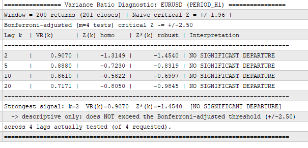
Running the script on EURUSD H1 with a 200-return window produces the following output:

5.1 Interpreting the VR Values

All four variance ratios are below 1, indicating that the observed variance grows more slowly than the random-walk benchmark across each tested horizon. The values also decrease as the lag increases: VR(2) is 0.907, VR(5) is 0.880, VR(10) is 0.861, and VR(20) is 0.711.

The largest departure from 1 occurs at k = 20, where the variance ratio is 0.711. This is the furthest of the four values from the random-walk benchmark. The shorter horizons also produce values below 1, although their departures are smaller. Taken together, the results show a progressively lower variance ratio across the tested horizons in this sample.

A VR below 1 indicates a net negative weighted sum of return autocorrelations up to lag k−1. However, the size of the departure alone does not tell us whether it is statistically significant. For that, we need to examine the corresponding test statistics.

5.2 Comparing the Test Statistics

The homoskedastic statistics are negative at all four horizons: Z(2) is -1.349, Z(5) is -0.730, Z(10) is -0.582, and Z(20) is -0.850. Each value remains within the naive critical range of ±1.96, so none reaches the conventional two-sided 5% significance threshold.

The heteroskedasticity-robust statistics show a similar pattern. Z*(2) is -1.450, Z*(5) is -0.819, Z*(10) is -0.699, and Z*(20) is -0.984. Their magnitudes are slightly larger than those of the corresponding homoskedastic statistics, but none exceeds the naive critical threshold of ±1.96.

The robust statistic is the primary reference here because financial returns often exhibit changing volatility. In this run, the adjustment does not change the interpretation: the results do not provide statistically significant evidence of a departure from random-walk variance scaling at any of the tested horizons.

5.3 Looking Across Multiple Horizons

The script tests four horizons: k = 2, 5, 10, and 20. Since multiple horizons are examined in the same run, the output also reports a Bonferroni-adjusted critical value of approximately ±2.50.

None of the robust statistics comes close to this adjusted threshold. The largest absolute robust statistic is 1.450 at k = 2, which remains below both the naive critical value of ±1.96 and the Bonferroni-adjusted value of ±2.50. The homoskedastic statistics also remain within both thresholds.

Although the variance ratios decrease as the horizon increases, this pattern is not accompanied by statistically significant test statistics. The observed departures may reflect sampling variation, and the results do not provide sufficient evidence to reject the random-walk variance-scaling null at any of the four tested horizons.

5.4 The Strongest Result

The script identifies k = 2 as the strongest signal because it has the largest absolute robust statistic among the tested horizons:

|Z*(2)| = 1.450

This is distinct from the largest variance-ratio departure, which occurs at k = 20. The variance ratio at k = 20 is furthest from 1, but its robust Z-statistic has a smaller absolute magnitude than the statistic at k = 2. The distinction matters because the Z-statistic accounts for estimated sampling variation, while the variance ratio shows only the direction and size of the variance-scaling departure.

Even the strongest statistic, at k = 2, does not reach the naive critical value of ±1.96, let alone the Bonferroni-adjusted threshold of ±2.50. It is therefore a descriptive result rather than a statistically significant finding. Selecting the largest statistic from several tested horizons does not, by itself, make that result significant.

5.5 What This Means for Trading

In this EURUSD H1 sample, the output does not provide statistically significant evidence of serial dependence at any of the four tested horizons. While all variance ratios are below 1, this alone is not sufficient to establish a reliable short-horizon reversal effect or a tradable mean-reversion opportunity.

The strongest statistical departure occurs at k = 2, but it remains below both the naive and Bonferroni-adjusted critical thresholds. The result should therefore be treated as an observed pattern in the selected sample, not as confirmation that the market is exhibiting a dependable mean-reverting structure.

The Variance Ratio test is a diagnostic for departures from random-walk variance scaling, not a complete trading signal. Any strategy built around a potential pattern would still require separate entry and exit logic, risk management, transaction-cost analysis, and out-of-sample validation before its practical value could be assessed.

6. Dropping the Engine Straight into an EA

The CVarianceRatio class can also be used directly inside an Expert Advisor. Since the engine has no chart objects, indicator buffers, or indicator handles to manage, the EA only needs to include the class and call its calculation method when the test is required. The example below shows how the Variance Ratio test can be used as one statistical input to a mean-reversion strategy's filter logic.

One caveat before the code: because this test re-runs every new bar on a rolling window that overlaps almost entirely with the previous bar's window, successive results are highly correlated with each other. This should be read as a slowly-updating regime diagnostic, not as a fresh, independent statistical test at every bar — treating a string of "significant" bars as repeated independent confirmation would understate the real uncertainty involved, a form of data snooping through repeated testing on overlapping data.

//+------------------------------------------------------------------+
//| Variance Ratio Test - Expert Advisor Example                     |
//+------------------------------------------------------------------+
#include <Quantitative/VarianceRatio.mqh>

//--- EA inputs
input int    InpWindowSize = 200;   // Number of returns in the test window
input int    InpLag        = 5;     // Aggregation horizon k
input double InpCriticalZ  = 1.96;  // One-sided threshold on Z* (1.96 ~ 2.5% one-sided level)

//--- Variance ratio test object
CVarianceRatio g_vr;

//+------------------------------------------------------------------+
//| Check whether a new bar has formed                               |
//+------------------------------------------------------------------+
bool IsNewBar()
  {
   static datetime last_bar_time = 0;

   datetime current_bar_time = iTime(_Symbol, _Period, 0);

   if(current_bar_time == 0)
      return false;

   if(current_bar_time != last_bar_time)
     {
      last_bar_time = current_bar_time;
      return true;
     }

   return false;
  }

//+------------------------------------------------------------------+
//| Test whether VR(k) is significantly below 1 at the chosen lag    |
//+------------------------------------------------------------------+
bool VarianceScalingBelowOne()
  {
   double vr;
   double z_homo;
   double z_hetero;

   //--- Build a chronological (oldest -> newest) close array, verified via
   //--- .time rather than assumed (see Section 4.2). start_pos = 1 uses
   //--- closed bars only, so the bar that just opened is excluded.
      int needed = g_vr.GetWindowSize() + 1; // window_size + 1 prices -> window_size returns
      MqlRates rates[];
      int copied = CopyRates(_Symbol, _Period, 1, needed + 10, rates);

      if(copied < needed)
         return false;

      bool alreadyChronological = (rates[0].time < rates[copied - 1].time);

      double closes[];
      ArrayResize(closes, copied);
      for(int i = 0; i < copied; i++)
         closes[i] = alreadyChronological ? rates[i].close : rates[copied - 1 - i].close;

   //--- Calculate the variance ratio and both test statistics
      if(!g_vr.Calculate(closes, InpLag, vr, z_homo, z_hetero))
         return false;

   //--- VR < 1: the weighted sum of autocorrelations up to lag k-1 is net negative.
   //--- The robust Z-statistic checks whether the departure from the
   //--- random-walk benchmark is large relative to its estimated variation.
      return (vr < 1.0 && z_hetero < -InpCriticalZ);
  }

//+------------------------------------------------------------------+
//| Expert initialization function                                   |
//+------------------------------------------------------------------+
int OnInit()
  {
   //--- Set the number of returns used by the variance ratio test
      g_vr.SetWindowSize(InpWindowSize);

      Print("Variance Ratio EA initialized.");
      PrintFormat("Window Size: %d | Lag: %d | Critical Z: %.2f",
                  g_vr.GetWindowSize(),
                  InpLag,
                  InpCriticalZ);

      return INIT_SUCCEEDED;
  }

//+------------------------------------------------------------------+
//| Expert tick function                                             |
//+------------------------------------------------------------------+
void OnTick()
  {
   //--- Run the test once per new bar
      if(!IsNewBar())
         return;

      if(VarianceScalingBelowOne())
        {
         //--- Proceed with the strategy's entry logic
            Print("VR(k) is significantly below 1 at this horizon.");
        }
      else
        {
            Print("No significant departure of VR(k) below 1 at this horizon.");
        }
  }
//+------------------------------------------------------------------+

Because the test fires on a new bar, starting the copy at position 1 means the bar that just closed is the last observation, rather than the bar that just opened.

The condition at the end of VarianceScalingBelowOne() combines two checks. VR(k) < 1 makes sure the net weighted autocorrelation is negative, while the robust Z-statistic checks whether that departure is large enough to be statistically significant. The EA requires both VR(k) < 1 and a robust Z-statistic below the negative critical threshold. In other words, the variance ratio must point below 1, and the robust statistic must provide enough evidence that the departure is unlikely to be explained by sampling variation alone. Note that z_hetero < -InpCriticalZ is a one-sided test, while 1.96 is the two-sided 5% critical value. Applied to one tail, it corresponds to a significance level of about 2.5%, stricter than a one-sided 5% test, which would use 1.645. That's a reasonable default for a filter, but it should be a choice you make knowingly.

The EA runs the test once per new bar to avoid redundant calculations. Note that this is a diagnostic filter, not a complete signal—a significantly low VR is compatible with mean-reversion assumptions, but it doesn't tell you when or how to trade. The VR < 1 check is explicit for readability, although a sufficiently negative Z-statistic already implies a VR below 1 when the estimated standard error is positive.

One more thing worth stating plainly before anyone points this at a live account: the lag k, the window size, and the critical-Z threshold used here need to be fixed ahead of time and validated out-of-sample, not tuned after looking at how well they would have performed. Picking a lag because it happened to look significant in a backtest — or widening the window until a favorable Z-statistic shows up — turns the statistical filter itself into just another curve-fitted trading rule, with all of the usual overfitting risk that implies. On top of that, a 200-return window at a single lag has limited statistical power to begin with, results can shift meaningfully from one window to the next, and this section hasn't touched transaction costs, execution, or slippage at all — none of which the test has any way of knowing about. Treat this example as showing how to wire the engine into an EA's decision logic, not as a validated trading rule on its own.

The actual entry logic remains separate from the statistical test. The Variance Ratio engine answers a narrower question: at the chosen horizon, is VR(k) significantly below 1, meaning the weighted sum of return autocorrelations is negative enough to be unlikely under the null? That is not the same as confirming a mean-reversion hypothesis, which VR, being a linear variance-scaling statistic, can't do on its own. That separation makes the class useful beyond this particular example. The same calculation can be used as a regime filter, a research component, or a diagnostic check without tying the statistical engine to any specific trading strategy — bearing in mind the rolling-retest caveat above whenever it's run continuously rather than as a one-off diagnostic.

7. Conclusion

We've implemented the Lo-MacKinlay Variance Ratio test as a reusable MQL5 component. The calculation engine can be reused inside EAs, while the diagnostic script provides a convenient way to explore the test interactively.

Remember, VR shows the direction of the variance-scaling departure, while Z indicates how large that departure is relative to its estimated sampling variation, provided the asymptotic approximation is adequate for the window used and the hypothesis was fixed in advance. When scanning multiple horizons, a Bonferroni- (or Holm-) adjusted threshold is the more honest bar to clear. For financial returns, the heteroskedasticity-robust statistic is usually the more appropriate one to emphasize, and, since this is a rolling-window diagnostic, a result should be read as evidence about the recent sample rather than fresh confirmation every time the window moves forward by one bar.

One natural extension left out here: printing an actual two-sided p-value alongside each Z-statistic, rather than only comparing against a fixed critical value, would make the output easier to read across several lags at once and would sit more comfortably next to the Bonferroni-adjusted alpha already being used. It wasn't essential to what this diagnostic sets out to do, so it's left as an exercise for anyone extending this further.

Attached files:

File Name	File Type	Description
VarianceRatio.mqh	Include file	Reusable calculation engine
VarianceRatioScript.mq5	Script	Multi-horizon diagnostic script
VarianceRatioEA.mq5	Expert Advisor (EA)	Example EA using the engine as a statistical filter