Measuring What Matters (Part 4): Reading the Spectrum — What Eigenvalues Tell You About Risk

Introduction

You already know how to build a covariance matrix and extract its eigenvalues. In Part 3, we validated that the eigenvectors and eigenvalues from .Eig() preserve the complete risk structure of the covariance matrix. The missing piece for practical trading is: what do those numbers tell you about portfolio risk in real situations - portfolio construction, ongoing monitoring, rebalancing, or enforcing risk limits? Three eigenvalues do not directly answer whether a portfolio is genuinely diversified or quietly riding on a single dominant risk driver. Instruments that look diverse by name or asset class can still have most of their variance absorbed by one volatility source or a shared market component.

This article fills that gap by applying spectral entropy to the eigenvalue spectrum and packaging the workflow in a reusable MQL5 script. The goal is explicit:

1. compress the full eigenvalue spectrum into a single comparable score,
2. enable direct portfolio-to-portfolio comparison,
3. provide a formal, thresholded alert when concentration becomes excessive.

SpectralEntropyCalculator.mq5 computes eigenvalues, converts them to variance proportions, calculates Shannon entropy normalized to [0,1] H_norm, reports the dominant-factor share, and issues a verdict - all reproducible for any two three-symbol portfolios.

What the Eigenvalue Spectrum Tells You

When you decompose the covariance matrix of a three-symbol portfolio you get three eigenvalues. Each eigenvalue represents the amount of variance carried by one independent risk factor — a direction in the portfolio’s risk space along which the instruments tend to move together. The sum of all eigenvalues gives the total variance represented by the covariance matrix. That identity is useful, but the real information sits in how the total is split among the individual eigenvalues.

Consider two possible outcomes.

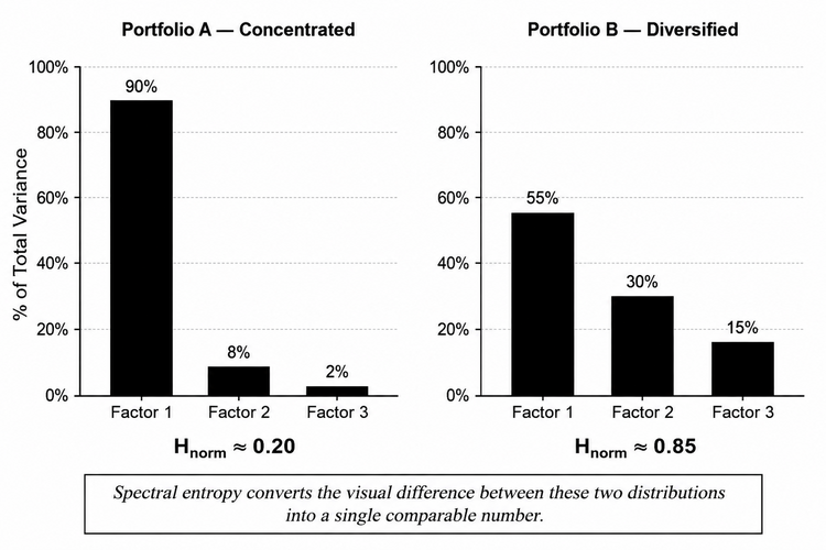
A concentrated spectrum might look something like 90 %, 8 %, 2 %. One factor is doing almost all the work. In practice this can mean that the instruments are heavily exposed to a common market force — dollar direction, broad risk sentiment, or commodity market tone. The other two factors are minor. Even though the portfolio holds three different instruments, they are mostly just different expressions of the same underlying bet. When that dominant factor moves sharply, the entire portfolio feels it. There is very little internal buffering.

A more distributed spectrum might look like 45 %, 35 %, 20 %. No single factor dominates. The variance is spread across three more evenly represented directions. When one factor jumps — a sudden dollar surge, for example — the other two can still remain relatively quiet and absorb some of the impact. That is closer to what genuine diversification looks like when viewed through eigenvalues. The portfolio has more than one engine, so a problem with one engine does not stop the whole machine.

You can often see the difference just by looking at the bars. One tall bar and two short ones versus three bars of roughly similar height. Most experienced traders develop an intuitive feel for this pattern after looking at enough portfolios. But visual inspection leaves a practical question: when does a dominant factor become excessive? Is 70 % acceptable? Is 80 % already dangerous? Spectral entropy is designed to answer that question with a single, comparable number instead of leaving the judgment entirely to the eye.

Spectral Entropy: A Single-Number Diversification Score

Spectral entropy takes the idea of Shannon entropy from information theory and applies it to the eigenvalue distribution. Shannon entropy measures how evenly a set of probabilities is spread: high when everything is roughly equal, low when one value dominates.

Here’s the process in four steps:

1. Decompose — extract the eigenvalues λ₁, λ₂, λ₃ with .Eig().
2. Normalize — turn each eigenvalue into a proportion of total variance: p[i] = λᵢ / Σλ. The proportions now sum to 1.0.
3. Shannon entropy — compute H = −Σ p[i] × log(p[i]). Proportions close to 0 or 1 drag the value down; equal proportions push it up.
4. Normalize to [0, 1] — divide H by log(n), where n is the number of factors. Now 1.0 means perfectly even distribution and 0.0 means everything sits in one factor, regardless of how many symbols you have. The final number, H_norm, is the diversification score.

Setting Up the Script: Two Portfolios, One Comparison

SpectralEntropyCalculator.mq5 is built around a comparison rather than a single portfolio. Looking at two portfolios side by side makes the entropy number far more useful than looking at it in isolation.

//--- Portfolio A inputs (concentrated — three correlated FX USD pairs)
input string          A_Symbol1     = "EURUSD";   // Portfolio A: Symbol 1
input string          A_Symbol2     = "GBPUSD";   // Portfolio A: Symbol 2
input string          A_Symbol3     = "AUDUSD";   // Portfolio A: Symbol 3

//--- Portfolio B inputs (diversified — FX, Gold, and an inverse pair)
input string          B_Symbol1     = "EURUSD";   // Portfolio B: Symbol 1
input string          B_Symbol2     = "XAUUSD";   // Portfolio B: Symbol 2
input string          B_Symbol3     = "USDJPY";   // Portfolio B: Symbol 3

//--- Shared parameters
input ENUM_TIMEFRAMES TF            = PERIOD_H1;  // Timeframe
input int             LookbackBars  = 100;        // Lookback period (bars)

//--- Entropy threshold: below this value the portfolio is flagged
input double          EntropyWarnThreshold = 0.75; // Entropy warning threshold (0-1)

Portfolio A starts with three USD pairs. All of them are heavily influenced by the same force — the US dollar. When the dollar moves, they tend to move together. On the surface it looks diversified; underneath it’s mostly one big dollar bet.

Portfolio B mixes EURUSD, XAUUSD and USDJPY. Gold responds to a different set of drivers (commodity flows, inflation, safe-haven demand), and USDJPY can behave differently during risk-off periods. On the surface, this looks like it should spread the variance more evenly.

The EntropyWarnThreshold defaults to 0.75. Anything below that gets a concentration warning. It is only a starting point, though. You can raise or lower it after looking at how the score behaves across your own portfolio and different market conditions.

The BuildCovMatrix Function: Encapsulating the Pipeline

Building the covariance matrix twice from scratch would be messy, so the whole pipeline is wrapped in one function:

//+------------------------------------------------------------------+
//| Build covariance matrix from three symbol return vectors         |
//+------------------------------------------------------------------+
bool BuildCovMatrix(const string &symbols[], int n,
                    ENUM_TIMEFRAMES tf, int bars,
                    matrix &cov_out)
  {
   vector returns[];
   ArrayResize(returns, n);

   for(int i = 0; i < n; i++)
      if(!ComputeLogReturns(symbols[i], tf, bars, returns[i]))
         return false;

   ulong cols = returns[0].Size();
   matrix all_returns;
   all_returns.Init(n, cols);
   for(int i = 0; i < n; i++)
      all_returns.Row(returns[i], i);

   cov_out = all_returns.Cov();

   if(cov_out.Rows() != (ulong)n || cov_out.Cols() != (ulong)n)
     {
      PrintFormat("ERROR: Unexpected matrix shape [%dx%d].",
                  cov_out.Rows(), cov_out.Cols());
      return false;
     }

   return true;
  }

You pass in the symbols, the count, the timeframe and the lookback; the function returns the covariance matrix by reference. Both portfolios are built with the same bars, so the comparison is fair.

Calling it is just:

if(!BuildCovMatrix(sym_a, 3, TF, LookbackBars, cov_a)) return;
if(!BuildCovMatrix(sym_b, 3, TF, LookbackBars, cov_b)) return;

The ComputeSpectralEntropy Function: Step by Step

This is the heart of the script. It takes a covariance matrix and returns the sorted eigenvalues, the proportions, the raw entropy, and the normalized score.

Decomposition and Total Variance

//+------------------------------------------------------------------+
//| Compute spectral entropy from a covariance matrix                |
//+------------------------------------------------------------------+
bool ComputeSpectralEntropy(const matrix &cov, int n,
                            vector &eigenvalues_out,
                            vector &proportions_out,
                            double &entropy_out,
                            double &entropy_norm_out)
  {
   matrix eigenvectors;
   vector eigenvalues;

   if(!cov.Eig(eigenvectors, eigenvalues))
     {
      Print("ERROR: Eigenvalue decomposition failed.");
      return false;
     }

//--- Compute total variance using native vector summation
   double total = eigenvalues.Sum();

.Eig() is called the same way as in earlier parts. eigenvalues.Sum() then gives the total variance in one clean call — no loop needed.

Sorting: Why ArraySort Instead of vector.Sort()

//--- Workaround: Use MQL5's native ArraySort() to avoid buggy vector.Sort()
   double eig_arr[];
   ArrayResize(eig_arr, n);
   for(int i = 0; i < n; i++)
      eig_arr[i] = eigenvalues[i];

   ArraySort(eig_arr); // Sorts ascending

//--- Read ascending array back into vector in descending order
   vector sorted_eigenvalues;
   sorted_eigenvalues.Init(n);
   for(int i = 0; i < n; i++)
      sorted_eigenvalues[i] = eig_arr[n - 1 - i];

MQL5’s vector .Sort() method has been unreliable in some builds with small vectors. Rather than risk a wrong order, the eigenvalues are copied into a normal double array, sorted with the solid ArraySort(), then read back in reverse so the largest comes first. Three extra lines, but the ordering is clear and predictable. That matters because the later warning looks at proportions[0] as the dominant factor.

Element-wise Vector Division for Proportions

//--- Compute proportions natively via element-wise vector division
   vector proportions = sorted_eigenvalues / total;

One line does the whole job. Dividing a vector by a scalar produces a new vector of proportions that sum to 1.0. The manual loop version works too, but the native operator is cleaner and closer to the mathematical notation.

One thing to keep in mind is that this calculation starts with a covariance matrix, so differences in the volatility of the instruments also affect the spectrum. A high-volatility instrument can take up a large share of the total variance even if it is not strongly correlated with the others. That becomes especially relevant when we look at the second portfolio later.

Shannon Entropy Calculation

//--- Calculate Shannon entropy
   double entropy = 0.0;
   for(int i = 0; i < n; i++)
     {
      if(proportions[i] > 0.0)
         entropy -= proportions[i] * MathLog(proportions[i]);
     }

//--- Normalize entropy to [0, 1] by dividing by log(n)
   double max_entropy = MathLog((double)n);
   double entropy_norm = (max_entropy > 0.0) ? entropy / max_entropy : 0.0;

The classic formula is H = −Σ p[i] × log(p[i]). The zero-guard is necessary because log(0) is undefined. Dividing by log(n) scales the result so that 1.0 always means maximum diversification and 0.0 means total concentration, no matter how many symbols you have.

The PrintEntropyReport Function: Making Entropy Readable

//+------------------------------------------------------------------+
//| Print full spectral entropy report for one portfolio             |
//+------------------------------------------------------------------+
void PrintEntropyReport(const string &symbols[], int n,
                        const string portfolio_label,
                        const vector &eigenvalues,
                        const vector &proportions,
                        double entropy,
                        double entropy_norm,
                        double warn_threshold)

This function turns the numbers into something a trader can scan quickly. It prints three parts: the eigenvalue table with a simple ASCII bar chart, the entropy calculation steps, and a clear verdict.

The bar chart is just asterisks — one for every 5 % of variance:

 //--- ASCII bar: each * = 5% of variance
      int bar_len = (int)MathRound(proportions[i] * 100.0 / 5.0);
      string bar  = "";
      for(int b = 0; b < bar_len; b++)
         bar += "*";

      PrintFormat("  Factor %d | lambda = %+.8f | %6.2f%% | %s",
                  i + 1, eigenvalues[i], proportions[i] * 100.0, bar);

A 90 % factor produces a long bar; a 10 % factor produces a short one. The contrast is visible even in plain text.

The calculation steps are printed so you can follow the numbers:

//--- Entropy calculation steps
   Print("  Entropy Calculation Steps:");
   PrintFormat("  Raw Shannon Entropy H      = %.6f nats", entropy);
   PrintFormat("  Maximum Entropy log(%d)     = %.6f nats", n, MathLog((double)n));
   PrintFormat("  Normalized Entropy H_norm  = %.6f  (%.2f%%)",
               entropy_norm, entropy_norm * 100.0);

Then the verdict:

//--- Verdict
   if(entropy_norm < warn_threshold)
     {
      PrintFormat("  WARNING: Portfolio is CONCENTRATED.");
      PrintFormat("  H_norm = %.4f — below threshold of %.2f.",
                  entropy_norm, warn_threshold);
      PrintFormat("  Dominant factor absorbs %.2f%% of total variance.",
                  proportions[0] * 100.0);
      PrintFormat("  Diversification is weaker than position sizing assumes.");
     }
   else
     {
      PrintFormat("  RESULT: Portfolio is DIVERSIFIED.");
      PrintFormat("  H_norm = %.4f — above threshold of %.2f.",
                  entropy_norm, warn_threshold);
      PrintFormat("  Variance is distributed across factors.");
     }

   PrintDivider("=");
  }

Because the eigenvalues were sorted descending, proportions[0] is always the biggest factor.

The PrintComparison Function: The Final Verdict

After both reports, a short summary puts the two H_norm values next to each other:

//+------------------------------------------------------------------+
//| Print side-by-side comparison of two portfolios                  |
//+------------------------------------------------------------------+
void PrintComparison(double entropy_a, double entropy_b,
                     const string label_a, const string label_b)
  {
   PrintDivider("=");
   Print("  PORTFOLIO COMPARISON SUMMARY");
   PrintDivider();
   PrintFormat("  %-30s | H_norm = %.4f (%.2f%%)",
               label_a, entropy_a, entropy_a * 100.0);
   PrintFormat("  %-30s | H_norm = %.4f (%.2f%%)",
               label_b, entropy_b, entropy_b * 100.0);
   PrintDivider();

   double diff = entropy_b - entropy_a;
   if(MathAbs(diff) < 0.01)
      Print("  RESULT: Both portfolios have similar diversification.");
   else
      if(diff > 0)
         PrintFormat("  RESULT: %s is MORE diversified by %.4f entropy units.",
                     label_b, diff);
      else
         PrintFormat("  RESULT: %s is MORE diversified by %.4f entropy units.",
                     label_a, MathAbs(diff));
  }

The labels are left-aligned so the numbers line up cleanly. A difference smaller than 0.01 is treated as effectively the same.

Reading the Output: What the Numbers Mean

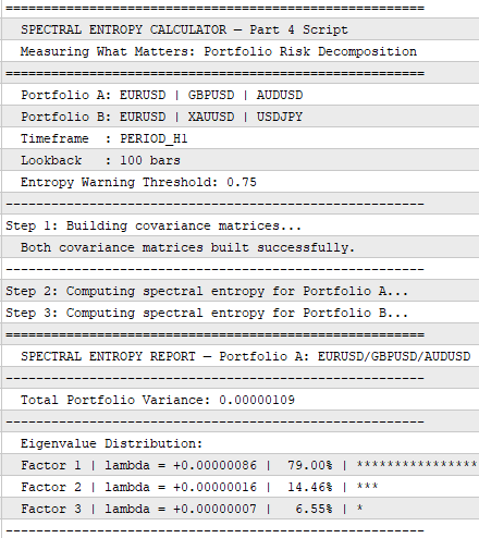
With the default inputs, the script produces two reports in the Expert Journal followed by a short comparison. The results are more interesting than the symbol names suggest.

Portfolio A — EURUSD / GBPUSD / AUDUSD Total variance ≈ 0.00000109

Factor 1 | lambda = +0.00000086 | 79.00% | ***************
Factor 2 | lambda = +0.00000016 | 14.46% | ***
Factor 3 | lambda = +0.00000007 |  6.55% | *

Factor 1 already accounts for 79 % of the total variance. The entropy numbers confirm the concentration:

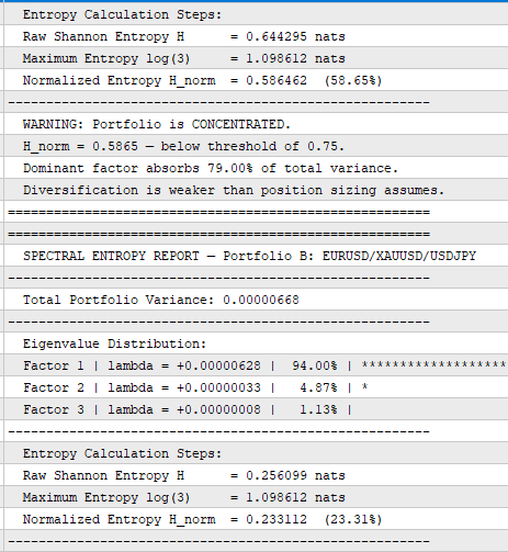
Raw Shannon Entropy H     = 0.644295 nats
Maximum Entropy log(3)    = 1.098612 nats
Normalized Entropy H_norm = 0.586462  (58.65%)

0.5865 sits below the 0.75 threshold, so the warning appears. Three dollar pairs are not three independent risks — the entropy score just makes that concrete.

Portfolio B — EURUSD / XAUUSD / USDJPY Total variance ≈ 0.00000668 (much larger, driven mostly by Gold)

Factor 1 | lambda = +0.00000628 | 94.00% | ********************
Factor 2 | lambda = +0.00000033 |  4.87% | *
Factor 3 | lambda = +0.00000008 |  1.13% |

Now Factor 1 takes 94 %. The entropy score drops even lower:

Raw Shannon Entropy H     = 0.256099 nats
Maximum Entropy log(3)    = 1.098612 nats
Normalized Entropy H_norm = 0.233112  (23.31%)

So the portfolio that looked more diversified by asset class is actually more concentrated in the variance structure captured by the covariance matrix. Gold's much larger variance takes up most of the spectrum.

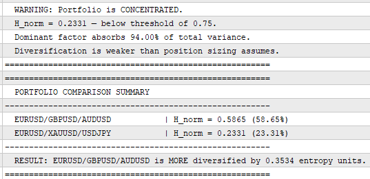
The final comparison line is blunt:

EURUSD/GBPUSD/AUDUSD  | H_norm = 0.5865 (58.65%)
EURUSD/XAUUSD/USDJPY  | H_norm = 0.2331 (23.31%)
RESULT: EURUSD/GBPUSD/AUDUSD is MORE diversified by 0.3534 entropy units.

Instrument names don’t decide diversification — the numbers do. Adding Gold doesn’t automatically make the variance more evenly distributed. What matters is whether the covariance structure is spread across several factors or dominated by one.

Change the LookbackBars input and watch how the scores shift in different market regimes. The 0.75 threshold is only a starting point. Over time, you can see what range of values is normal for your portfolio and when the score starts to signal unusual concentration.

Conclusion

Eigenvalues by themselves are raw measurements; spectral entropy converts that spectrum into an actionable diversification score. Part 3 established that these eigenvalues and their corresponding eigenvectors faithfully reconstruct the covariance matrix, giving us confidence that the spectrum represents the portfolio's complete risk structure. Using the pipeline in this article you obtain, for each three-symbol portfolio: sorted eigenvalues, each factor's share of total variance, raw Shannon entropy, and a normalized H_norm in [0,1]. The script also prints the dominant factor's percentage, a simple ASCII bar chart for quick inspection, and a threshold-based verdict so you can flag concentrated portfolios automatically.

Practically, SpectralEntropyCalculator.mq5 gives you a repeatable test you can run on any two portfolios to see which one spreads variance more evenly. Remember two caveats: covariance captures both correlation and relative volatility (a very volatile instrument can dominate the spectrum), and the default threshold (0.75) is a starting point that should be calibrated to your asset mix and time horizons. Use the score for selection, routine monitoring, rebalancing signals, or guardrails in risk limits. The natural next step is operationalizing this into a live indicator that plots H_norm over time so you can watch concentration build or diversification erade in real time.

Next: Part 5 — The Risk Concentration Indicator