Measuring What Matters (Part 5): The Risk Concentration Indicator — Plotting Eigenvalue Dominance Live
 142
 0

Introduction
Every script built in this series so far has answered a question about a fixed window of historical data. You run it, you read the output, you close it. That is useful for understanding the risk structure of a portfolio at a point in time. It is not useful for trading, because risk concentration does not stay fixed. The estimated covariance relationships between instruments change as the rolling window moves through different market regimes — correlations spike during macro events, compress during quiet periods, and reverse during risk-off episodes. A trader who checks their portfolio's eigenvalue spectrum once a week may be carrying substantially higher risk concentration for days before they detect the change.
Part 5 solves this by converting the eigenvalue analysis into a live indicator. RiskConcentrationIndicator.mq5 plots the dominant eigenvalue's percentage of total portfolio variance as a continuous histogram in a separate window — blue bars when concentration is within acceptable bounds, red bars when it has crossed the alert threshold. The histogram updates on each calculated bar, giving the trader a continuous view of how concentrated their portfolio risk is over time.
It's worth being precise about what "portfolio" means here: the calculation treats the three instruments as an equally-weighted, unit-exposure basket. It measures how concentrated the variance is within the covariance structure of the three return series themselves — not in a specific portfolio's actual position sizes, currency exposures, or contract multipliers. That layer is what Part 6 adds when it turns the eigenvectors into position weights.
The final implementation introduces a rolling prefix sum engine. Persistent global arrays accumulate running sums of returns, squared returns, and cross-products, so each new bar extends the covariance state without re-pulling or re-scanning the full lookback window. It introduces timestamp-based symbol alignment using iBarShift(). Each instrument is matched by the chart bar's timestamp rather than a numerical bar index. An exact-match rule rejects any case where a symbol has no bar opening at that precise time, or where the bar before it is not the chart’s previous bar. It also introduces principled missing-data handling. Bars are excluded when any symbol's return cannot be fetched (instead of being zero-filled). A valid-count prefix tracks the true sample size and computation blocks when gaps exceed the allowed fraction. The result is an indicator designed to operate efficiently on a live chart while accounting for incomplete and asynchronous market data. The indicator supports one operating mode: CalcTimeframe must equal the chart’s timeframe, and OnInit() enforces it.
From Script to Indicator: The Structural Difference
The scripts in Parts 1 through Part 4 all used OnStart() — a function that executes once from top to bottom and exits. An indicator uses OnCalculate() — a function that the terminal calls on every new tick and every new bar, passing the current state of the chart's price arrays. The indicator persists for as long as it is attached to the chart, maintaining its own state between calls.
This difference has direct consequences for how the covariance calculation must be designed. A script can afford to pull LookbackBars of price data on every run because it only runs once. An indicator running OnCalculate() on every bar cannot re-pull and re-process 100 bars of data for three symbols on every tick — the computational cost would make the terminal sluggish and the indicator impractical on any chart with significant history.
The solution is the rolling prefix sum engine. Instead of recomputing the covariance matrix from scratch on every bar, the indicator maintains running totals that extend in one operation per bar and recovers any windowed statistic via a simple subtraction. Windowed covariance statistics can be recovered from prefix sums in O(1) time with respect to lookback length. This bound applies only to recovering window statistics from the running totals. It does not cover the cost of extending totals by one bar. Each extension still requires an iBarShift() lookup and a CopyClose() call per symbol. That per-bar cost is constant with respect to LookbackBars — it doesn't grow as the window gets longer — but it isn't free: it still depends on the terminal having quick access to each symbol's price history.
Indicator Properties and Inputs
The property block sets up a three-buffer, three-plot indicator in a separate window with a fixed scale, and declares the label, type, color, style and width of each plot:
#property indicator_separate_window
#property indicator_buffers 3
#property indicator_plots   3

#property indicator_minimum 0.0
#property indicator_maximum 100.0

//--- Plot 0: Safe bars (blue) - concentration below alert level
#property indicator_label1  "Safe Zone"
#property indicator_type1   DRAW_HISTOGRAM
#property indicator_color1  clrDodgerBlue
#property indicator_style1  STYLE_SOLID
#property indicator_width1  3

//--- Plot 1: Danger bars (red) - concentration at or above alert level
#property indicator_label2  "Concentrated"
#property indicator_type2   DRAW_HISTOGRAM
#property indicator_color2  clrRed
#property indicator_style2  STYLE_SOLID
#property indicator_width2  3

//--- Plot 2: Alert level line
#property indicator_label3  "Alert Level"
#property indicator_type3   DRAW_LINE
#property indicator_color3  clrDarkRed
#property indicator_style3  STYLE_DOT
#property indicator_width3  1
indicator_minimum and indicator_maximum fix the scale of the indicator's own sub-window to 0-100% permanently. This is the correct approach for a sub-window indicator — unlike ChartSetInteger() which would incorrectly target the main chart window and break the candlestick display.
Three plots are declared: a blue histogram for concentration levels below the alert threshold, a red histogram for levels at or above it, and a dotted line marking the AlertLevel threshold itself. The two histogram plots use DRAW_HISTOGRAM — bars drawn from the zero baseline upward — and indicator_width1/2 of 3 for visible bar thickness; the third plot uses DRAW_LINE at width 1 to trace a constant reference line at the chosen alert percentage, so the boundary between the blue and red bars is visible on the chart rather than left for the trader to remember.
The inputs introduce two new parameters beyond what the previous scripts used:
input int             RecalcEveryBars      = 1;         // Recalculate eigen-decomposition every N bars
input double          MinValidDataFraction = 0.70;      // Min valid-data fraction in window - heuristic starting value
RecalcEveryBars throttles the eigenvalue decomposition — the most computationally expensive step — on closed, historical bars, recalculating only every N bars while the cheaper prefix sum update runs on every bar. The current, still-forming bar is an exception: it always gets a fresh eigendecomposition on every tick regardless of RecalcEveryBars, keeping the live reading responsive to the bar that's actually moving. MinValidDataFraction sets the minimum fraction of the lookback window that must contain valid data before the indicator will compute a fresh concentration reading. If more than 30% of the window is missing data, the indicator withholds a fresh reading for that bar — whether the chart then shows an empty bar or the last carried-forward value depends on whether a valid reading was ever computed earlier, as the OnCalculate walkthrough below explains. The defaults for AlertLevel (70.0) and MinValidDataFraction (0.70) are illustrative starting points rather than calibrated values. The section on reading the indicator explains how to think about adjusting them.
CalcTimeframe Must Match the Chart Timeframe
One constraint underpins the rest of the design. OnCalculate() builds one prefix-sum row for every bar on the chart, keyed to that bar’s timestamp, while GetAlignedLogReturn() reads each symbol’s data on CalcTimeframe. The two only describe the same sequence of bars when CalcTimeframe equals the chart’s timeframe.
If they differ, the results break in one of two ways. With a nearest-bar match, several consecutive chart bars fall inside the same higher-timeframe bar, so the same return is added to the prefix sums more than once and the valid count is inflated. With the exact-time match used here, most chart bars find no bar opening at their timestamp and are excluded as gaps. Neither produces a meaningful covariance estimate.
Rather than maintain a second time axis, the indicator supports a single mode and enforces it. OnInit() returns INIT_PARAMETERS_INCORRECT and logs a message when CalcTimeframe differs from the chart’s timeframe. To analyze a different timeframe, attach the indicator to a chart of that timeframe and set CalcTimeframe to match. Driving the loop from CalcTimeframe bars instead of the chart’s time[] array would lift the restriction, but that is outside the scope of this article.
The Global Prefix Sum State
The rolling engine is built on persistent global arrays declared at file scope:
//--- Persistent rolling-sum state (grows as new bars arrive, never rebuilt from scratch)
double g_pfxR1[],  g_pfxR2[],  g_pfxR3[];      // prefix sums of returns per symbol
double g_pfxR1R1[], g_pfxR2R2[], g_pfxR3R3[];  // prefix sums of squared returns
double g_pfxR1R2[], g_pfxR1R3[], g_pfxR2R3[];  // prefix sums of cross-products
int    g_pfxValid[];                           // prefix COUNT of bars where all 3 returns were valid
int    g_pfxSize = 0;                          // current capacity of the prefix arrays

int    g_consecutiveFailures = 0;              // throttles diagnostic prints
int    g_lastFailedBarIndex  = -1;             // avoids double-counting the same bar across ticks
The first three arrays accumulate the running sum of log returns for each symbol. The next three accumulate the running sum of squared returns — the raw material for computing variance. The final three accumulate the running sum of cross-products between each symbol pair — the raw material for covariance. g_pfxValid counts how many bars in the running total contained valid data from all three symbols. g_pfxSize tracks the current allocated capacity so arrays are only grown when needed. g_consecutiveFailures and g_lastFailedBarIndex track diagnostic state for missing-data gaps — covered in detail when UpdatePrefixSumsAtBar() is introduced below.
Together these prefix arrays contain everything required to compute the mean and population covariance of any sub-window of the history in O(1) time with respect to the window length — without touching any price data. The covariance of the window from bar (i-n+1) to bar i is recovered by subtracting the prefix sum at position (i-n) from the prefix sum at position i.
EnsurePrefixCapacity: Growing Arrays on Demand
//+------------------------------------------------------------------+
//| Grow the persistent prefix-sum arrays to at least `size`         |
//+------------------------------------------------------------------+
void EnsurePrefixCapacity(int size)
  {
   if(size <= g_pfxSize)
      return;

   ArrayResize(g_pfxR1,  size);
   ArrayResize(g_pfxR2,  size);
   ArrayResize(g_pfxR3,  size);
   ArrayResize(g_pfxR1R1, size);
   ArrayResize(g_pfxR2R2, size);
   ArrayResize(g_pfxR3R3, size);
   ArrayResize(g_pfxR1R2, size);
   ArrayResize(g_pfxR1R3, size);
   ArrayResize(g_pfxR2R3, size);
   ArrayResize(g_pfxValid, size);

   g_pfxSize = size;
  }
This function is called at the start of every OnCalculate() with rates_total as its argument. If the chart has more bars than the arrays currently hold, all ten arrays are resized to accommodate. If the arrays are already large enough, the function returns immediately without any allocation. This means memory is only allocated when the chart history grows — typically once on startup and occasionally after a chart reload.
GetAlignedLogReturn: Timestamp-Based Symbol Alignment
The function that fetches a single log return for one symbol is the foundation of the alignment strategy:
//+-------------------------------------------------------------------+
//| Fetch a single log return for `symbol`, ln(P_t / P_{t-1}), aligned|
//| to the CHART's timestamps. Alignment is EXACT at BOTH ends of the |
//| return (time tolerance = 0 seconds):                              |
//|   - the symbol must have a bar opening at `barTime` (price P_t);  |
//|   - the bar immediately before it must open at `prevBarTime`,     |
//|     the chart's previous bar time (price P_{t-1}).                |
//| A neighbouring bar is never accepted in place of a missing one,   |
//| and a return is never stretched over a missing bar. Returns false |
//| if either condition fails.                                        |
//+-------------------------------------------------------------------+
bool GetAlignedLogReturn(const string symbol, ENUM_TIMEFRAMES tf,
                         datetime barTime, datetime prevBarTime, double &ret)
  {
   int shift = iBarShift(symbol, tf, barTime, true);   // exact match only
   if(shift < 0)
      return false;

//--- Defensive re-check: the bar found must open exactly at barTime.
   if(iTime(symbol, tf, shift) != barTime)
      return false;

//--- The bar before it must be the chart's previous bar. If the symbol
//--- skipped a bar, CopyClose() below would return a close from further
//--- back and the return would span more than one bar.
   if(iTime(symbol, tf, shift + 1) != prevBarTime)
      return false;

   double price[];
   ArraySetAsSeries(price, true);

   if(CopyClose(symbol, tf, shift, 2, price) != 2)
      return false;

   if(price[0] <= 0.0 || price[1] <= 0.0)
      return false; // treat non-positive close as missing/corrupt data, not a real 0% return

   ret = MathLog(price[0] / price[1]);
   return true;
  }
The critical design decision is the exact = true argument to iBarShift(). A symbol’s bar counts as aligned only if it opens at exactly the same time as the chart bar, so the time tolerance is zero seconds. Bar open times are normalized to the timeframe boundary, which means two symbols that both traded in a given period share the same open time and no small offset needs to be allowed for. The iTime() comparison that follows is a defensive re-check, and a symbol with no bar at that time is treated as missing.
A looser rule, accepting the nearest bar and rejecting only differences larger than one bar period, would leave a single-bar-skip hole, because a difference of exactly one period would pass. Suppose Gold has no 10:00 bar on an H1 chart while EURUSD and GBPUSD do. A nearest-bar lookup returns Gold’s 09:00 bar, exactly 3600 seconds away, and that rule would accept it as the 10:00 observation. The same thing could happen on the forming bar before a symbol’s first tick of the new period arrives. Under the exact-match rule, the 10:00 bar is excluded for all three symbols instead: the sums and valid count carry forward, and the gap is logged.
This matters because different instruments can have different trading sessions and holiday calendars. XAUUSD, for example, does not necessarily have the same available bars as EURUSD. Only a bar that opens at exactly the chart bar’s time counts as aligned, which also means the forming bar can be briefly excluded until every symbol has ticked in the new period.
The exact match is applied at both ends of the return. A log return is ln(P_t / P_{t-1}), so aligning only the bar at t would leave the second price unchecked: if a symbol has a bar at barTime but is missing the bar before it, CopyClose() would return a close from further back, and a return stretched over more than one bar would enter the covariance matrix as if it were an ordinary one-bar return. To prevent that, the function also receives prevBarTime, the open time of the chart’s own previous bar, and requires the symbol’s preceding bar to open at exactly that time. Using the chart’s previous bar rather than barTime minus one period keeps the rule independent of the calendar: a weekend closure shared by all three symbols is not treated as a gap, because each symbol’s preceding bar is the same last bar before the closure. The consequence is deliberate. The first bar after a gap in any one symbol is excluded, because its return would cover more than one bar for that symbol.
The ArraySetAsSeries(price, true) call ensures that price[0] is the most recent close and price[1] is the preceding close, giving the log return ln(P_t / P_{t-1}). Non-positive prices return false immediately — treated as missing or corrupt data rather than a real zero-percent return.
UpdatePrefixSumsAtBar: The O(1) Rolling Update
This function is called for every bar in OnCalculate(). It is the engine that makes the rolling covariance possible:
//+------------------------------------------------------------------+
//| Extend the rolling prefix sums by exactly one bar (index i).     |
//| `prevBarTime` is the chart's previous bar time (time[i-1]).      |
//| All three symbols must be valid, or the whole bar is excluded    |
//| (sums and valid-count both carried forward unchanged) so a gap   |
//| in one symbol never gets silently treated as a 0.0 return.       |
//| Bar 0 has no preceding chart bar, so it carries no return; that  |
//| is not a data gap and is not logged as one.                      |
//+------------------------------------------------------------------+
void UpdatePrefixSumsAtBar(int i, datetime barTime, datetime prevBarTime)
  {
   double r1, r2, r3;
   bool ok = (i > 0)
             && GetAlignedLogReturn(Symbol1, CalcTimeframe, barTime, prevBarTime, r1)
             && GetAlignedLogReturn(Symbol2, CalcTimeframe, barTime, prevBarTime, r2)
             && GetAlignedLogReturn(Symbol3, CalcTimeframe, barTime, prevBarTime, r3);

   double prevR1  = (i > 0) ? g_pfxR1[i-1]  : 0.0;
   double prevR2  = (i > 0) ? g_pfxR2[i-1]  : 0.0;
   double prevR3  = (i > 0) ? g_pfxR3[i-1]  : 0.0;
   double prevR1R1 = (i > 0) ? g_pfxR1R1[i-1] : 0.0;
   double prevR2R2 = (i > 0) ? g_pfxR2R2[i-1] : 0.0;
   double prevR3R3 = (i > 0) ? g_pfxR3R3[i-1] : 0.0;
   double prevR1R2 = (i > 0) ? g_pfxR1R2[i-1] : 0.0;
   double prevR1R3 = (i > 0) ? g_pfxR1R3[i-1] : 0.0;
   double prevR2R3 = (i > 0) ? g_pfxR2R3[i-1] : 0.0;
   int    prevValid = (i > 0) ? g_pfxValid[i-1] : 0;

   if(!ok)
     {
      //--- Excluded bar: sums and valid-count carried forward untouched.
      g_pfxR1[i] = prevR1;
      g_pfxR2[i] = prevR2;
      g_pfxR3[i] = prevR3;
      g_pfxR1R1[i] = prevR1R1;
      g_pfxR2R2[i] = prevR2R2;
      g_pfxR3R3[i] = prevR3R3;
      g_pfxR1R2[i] = prevR1R2;
      g_pfxR1R3[i] = prevR1R3;
      g_pfxR2R3[i] = prevR2R3;
      g_pfxValid[i] = prevValid;

      //--- Only count this as a NEW gap the first time this bar index
      //--- fails. A live/forming bar can be re-evaluated many times
      //--- per tick, and none of those re-evaluations are new gaps.
      if(i > 0 && i != g_lastFailedBarIndex)
        {
         g_consecutiveFailures++;
         g_lastFailedBarIndex = i;
         if(g_consecutiveFailures == 1 || g_consecutiveFailures % 500 == 0)
            PrintFormat("RiskConcentrationIndicator: missing/unusable data for one or more symbols at %s (consecutive gaps: %d)",
                        TimeToString(barTime), g_consecutiveFailures);
        }
      return;
     }

   g_consecutiveFailures = 0;
   g_lastFailedBarIndex  = -1;

   g_pfxR1[i]  = prevR1  + r1;
   g_pfxR2[i]  = prevR2  + r2;
   g_pfxR3[i]  = prevR3  + r3;
   g_pfxR1R1[i] = prevR1R1 + r1 * r1;
   g_pfxR2R2[i] = prevR2R2 + r2 * r2;
   g_pfxR3R3[i] = prevR3R3 + r3 * r3;
   g_pfxR1R2[i] = prevR1R2 + r1 * r2;
   g_pfxR1R3[i] = prevR1R3 + r1 * r3;
   g_pfxR2R3[i] = prevR2R3 + r2 * r3;
   g_pfxValid[i] = prevValid + 1;
  }
The function attempts to fetch aligned log returns for all three symbols at barTime. If all three succeed, it adds each return and each cross-product to the running totals and increments the valid count. If any one symbol fails — because the symbol has no bar at that timestamp, its preceding bar is not the chart’s previous bar, or the price is corrupt — the entire bar is excluded. All sums are carried forward unchanged, and the valid count stays the same. The bar is treated as if it did not exist. Bar 0 has no preceding chart bar, so it carries no return; it is carried forward like an excluded bar but is not logged as a data gap.
This is the principled approach to missing data. Zero-filling a missing return — using 0.0 when a symbol has no data — would artificially reduce the estimated variance of that symbol and distort all covariances involving it. By carrying forward unchanged sums instead, the valid-bar window correctly reflects only the bars where all three symbols had real, usable prices.
The g_consecutiveFailures counter throttles diagnostic printing, but it only advances the first time a given bar index fails — the current bar can be re-evaluated many times within a tick, or across many ticks before it closes, and none of those re-evaluations should count as a new gap. g_lastFailedBarIndex tracks which bar the last failure belonged to, so a bar that keeps failing while it's still forming is logged once, not once per tick. The first genuinely new gap prints immediately; subsequent consecutive gaps only print every 500 bars — preventing a flood of journal messages if a symbol is missing data for an extended period.
BuildWindowCovariance: O(1) Covariance from Prefix Differences
With the prefix sums in place, recovering the covariance matrix for any window is a simple subtraction:
//+------------------------------------------------------------------+
//| Recover the windowed covariance matrix from the prefix sums via  |
//| a simple difference. Uses the ACTUAL valid sample count in the   |
//| window (not the raw bar-window size) for the mean/covariance     |
//| divisor, and refuses to compute if too much of the window is     |
//| missing data.                                                    |
//+------------------------------------------------------------------+
bool BuildWindowCovariance(int i, int n, matrix &cov)
  {
   if(i - n + 1 < 0)
      return false;

   int validCount = (i - n >= 0) ? (g_pfxValid[i] - g_pfxValid[i-n]) : g_pfxValid[i];

   int minRequired = (int)MathCeil(n * MinValidDataFraction);
   if(minRequired < 2)
      minRequired = 2;
   if(validCount < minRequired)
      return false;

   double sumR1, sumR2, sumR3, sumR1R1, sumR2R2, sumR3R3, sumR1R2, sumR1R3, sumR2R3;

   if(i - n >= 0)
     {
      sumR1   = g_pfxR1[i]   - g_pfxR1[i-n];
      sumR2   = g_pfxR2[i]   - g_pfxR2[i-n];
      sumR3   = g_pfxR3[i]   - g_pfxR3[i-n];
      sumR1R1 = g_pfxR1R1[i] - g_pfxR1R1[i-n];
      sumR2R2 = g_pfxR2R2[i] - g_pfxR2R2[i-n];
      sumR3R3 = g_pfxR3R3[i] - g_pfxR3R3[i-n];
      sumR1R2 = g_pfxR1R2[i] - g_pfxR1R2[i-n];
      sumR1R3 = g_pfxR1R3[i] - g_pfxR1R3[i-n];
      sumR2R3 = g_pfxR2R3[i] - g_pfxR2R3[i-n];
     }
   else
     {
      sumR1   = g_pfxR1[i];
      sumR2   = g_pfxR2[i];
      sumR3   = g_pfxR3[i];
      sumR1R1 = g_pfxR1R1[i];
      sumR2R2 = g_pfxR2R2[i];
      sumR3R3 = g_pfxR3R3[i];
      sumR1R2 = g_pfxR1R2[i];
      sumR1R3 = g_pfxR1R3[i];
      sumR2R3 = g_pfxR2R3[i];
     }

   double n_eff = (double)validCount; // true sample size, excluding gaps

   double meanR1 = sumR1 / n_eff;
   double meanR2 = sumR2 / n_eff;
   double meanR3 = sumR3 / n_eff;

//--- Population covariance over the valid points only. A constant
//--- scale factor here does not affect the eigenvalue-share-of-trace
//--- percentage we ultimately plot. Diagonal terms are clamped to
//--- guard against tiny negative variances from floating-point
//--- rounding in E[X^2] - E[X]^2.
   cov.Init(3, 3);
   cov[0][0] = MathMax(sumR1R1 / n_eff - meanR1 * meanR1, 0.0);
   cov[1][1] = MathMax(sumR2R2 / n_eff - meanR2 * meanR2, 0.0);
   cov[2][2] = MathMax(sumR3R3 / n_eff - meanR3 * meanR3, 0.0);
   cov[0][1] = cov[1][0] = sumR1R2 / n_eff - meanR1 * meanR2;
   cov[0][2] = cov[2][0] = sumR1R3 / n_eff - meanR1 * meanR3;
   cov[1][2] = cov[2][1] = sumR2R3 / n_eff - meanR2 * meanR3;

   return true;
  }
The window from bar (i-n+1) to bar i is extracted by subtracting the prefix value at position (i-n) from the prefix value at position i. This is the standard prefix sum trick: if g_pfxR1[i] is the total of all returns from bar 0 to bar i, then g_pfxR1[i] - g_pfxR1[i-n] is the total of all returns from bar (i-n+1) to bar i — exactly the LookbackBars window.
The valid count for the window is recovered the same way. minRequired ensures the window has enough real data: if MinValidDataFraction is 0.70 and LookbackBars is 100, at least 70 bars must have valid data from all three symbols. If fewer than 70 are valid, the function returns false — though that only means this function produced nothing; whether the chart shows an empty bar or carries forward the last valid reading is decided further down in OnCalculate().
The covariance formula uses n_eff — the actual valid count — as the divisor rather than the raw window size n. This gives the correct population mean and covariance over the valid data points, not a diluted estimate that treats missing bars as zero-return bars.
A note on the formula: the code uses the computational form of variance — E[X²] - (E[X])² — which avoids a second pass over the data and works directly from the prefix sums. The result is a population covariance, which shares the same eigenvalue-share-of-trace percentage as the sample covariance. The constant scale factor between population and sample covariance cancels out when computing the dominant eigenvalue as a percentage of total variance.
There's a numerical wrinkle worth flagging here: E[X²] − E[X]² is mathematically always non-negative for a real variance, but computed in floating point it can drift slightly below zero when the true variance is near zero and the two terms nearly cancel. Left unguarded, that surfaces downstream as a negative eigenvalue or a concentration percentage that overshoots 100%. The diagonal terms are clamped to zero for exactly that reason, and ComputeConcentration() applies the same clamp to the eigenvalues before summing them.
ComputeConcentration: Eigendecomposition and Dominant Factor
//+------------------------------------------------------------------+
//| Dominant eigenvalue as a percentage of total variance (trace).   |
//| Eigenvalues are clamped to zero before use - the same rounding-  |
//| error guard applied to the covariance diagonal - and the final   |
//| percentage is capped at 100 so residual noise can't push the     |
//| plotted value past the indicator's fixed scale.                  |
//+------------------------------------------------------------------+
double ComputeConcentration(int i, int n)
  {
   matrix cov;
   if(!BuildWindowCovariance(i, n, cov))
      return -1.0;

   matrix eigenvectors;
   vector eigenvalues;
   if(!cov.Eig(eigenvectors, eigenvalues))
      return -1.0;

   double total = 0.0;
   for(int k = 0; k < (int)eigenvalues.Size(); k++)
      total += MathMax(eigenvalues[k], 0.0);
   if(total <= 0.0)
      return -1.0;

   double maxEig = 0.0;
   for(int k = 0; k < (int)eigenvalues.Size(); k++)
     {
      double e = MathMax(eigenvalues[k], 0.0);
      if(e > maxEig)
         maxEig = e;
     }

   return MathMin((maxEig / total) * 100.0, 100.0);
  }
This function calls BuildWindowCovariance to recover the covariance matrix from the prefix sums, then calls.Eig() to decompose it. Each eigenvalue is clamped to zero before use, for the same rounding-error reason the covariance diagonal is clamped — a covariance matrix built from noisy floating-point sums can occasionally produce a tiny negative eigenvalue where the true value is zero. The dominant eigenvalue is found with a simple linear scan — a direct loop over the three eigenvalues comparing each to the current maximum. This replaces the ArraySort() workaround used in earlier parts of this series. For a three-element eigenvalue vector, a three-iteration scan is both simpler and more transparent than copying to a double array and sorting. The result — the dominant eigenvalue divided by the total variance, expressed as a percentage — is also capped at 100%, so the same rounding noise can't push the plotted value past the top of the indicator's fixed scale.
OnInit: Buffer Binding and State Reset
//+------------------------------------------------------------------+
//| Custom indicator initialization                                  |
//+------------------------------------------------------------------+
int OnInit()
  {
//--- Validate inputs before doing anything else. An indicator that
//--- loads with a nonsensical setting can misbehave silently, so
//--- these fail fast with a clear reason in the Experts log.
   if(RecalcEveryBars <= 0)
     {
      Print("RiskConcentrationIndicator: RecalcEveryBars must be >= 1.");
      return INIT_PARAMETERS_INCORRECT;
     }
   if(LookbackBars <= 1)
     {
      Print("RiskConcentrationIndicator: LookbackBars must be >= 2.");
      return INIT_PARAMETERS_INCORRECT;
     }
   if(MinValidDataFraction <= 0.0 || MinValidDataFraction > 1.0)
     {
      Print("RiskConcentrationIndicator: MinValidDataFraction must be in (0, 1].");
      return INIT_PARAMETERS_INCORRECT;
     }
   if(AlertLevel < 0.0 || AlertLevel > 100.0)
     {
      Print("RiskConcentrationIndicator: AlertLevel must be in the range 0-100%.");
      return INIT_PARAMETERS_INCORRECT;
     }

//--- Supported mode: the prefix sums are built on the chart's own bars
//--- (time[i]) while symbol data is read on CalcTimeframe, so the two
//--- must be the same timeframe.
   if(CalcTimeframe != (ENUM_TIMEFRAMES)Period())
     {
      PrintFormat("RiskConcentrationIndicator: CalcTimeframe (%s) must equal the chart timeframe (%s). Attach the indicator to a %s chart.",
                  EnumToString(CalcTimeframe),
                  EnumToString((ENUM_TIMEFRAMES)Period()),
                  EnumToString(CalcTimeframe));
      return INIT_PARAMETERS_INCORRECT;
     }

   SetIndexBuffer(0, SafeBuffer,   INDICATOR_DATA);
   SetIndexBuffer(1, DangerBuffer, INDICATOR_DATA);
   SetIndexBuffer(2, AlertBuffer,  INDICATOR_DATA);

//--- Indexing invariant: buffers are chronological (index 0 = oldest
//--- bar), the same direction as the time[] array in OnCalculate().
   ArraySetAsSeries(SafeBuffer,   false);
   ArraySetAsSeries(DangerBuffer, false);
   ArraySetAsSeries(AlertBuffer,  false);

//--- Empty value: EMPTY_VALUE hides the bar entirely when not drawn.
//--- The alert line always receives a real AlertLevel value in
//--- OnCalculate(), so its empty-value setting only matters in the
//--- edge case where AlertLevel itself is exactly 0.
   PlotIndexSetDouble(0, PLOT_EMPTY_VALUE, EMPTY_VALUE);
   PlotIndexSetDouble(1, PLOT_EMPTY_VALUE, EMPTY_VALUE);
   PlotIndexSetDouble(2, PLOT_EMPTY_VALUE, EMPTY_VALUE);

   IndicatorSetString(INDICATOR_SHORTNAME,
                      StringFormat("Risk Concentration [%s/%s/%s] L:%d Alert:%.0f%%",
                                   Symbol1, Symbol2, Symbol3,
                                   LookbackBars, AlertLevel));
   IndicatorSetInteger(INDICATOR_DIGITS, 2);

   g_pfxSize = 0;             // force prefix arrays to be (re)built from bar 0
   g_consecutiveFailures = 0;
   g_lastFailedBarIndex  = -1;

   return INIT_SUCCEEDED;
  }
Before any buffers are bound, OnInit() checks the four inputs that could otherwise break the indicator silently, along with the chart timeframe. RecalcEveryBars must be at least 1, since the modulo throttle in OnCalculate() would divide by zero otherwise. LookbackBars must be at least 2, or the covariance calculation has no statistical basis. MinValidDataFraction must fall inside (0, 1] — above 1 no window could ever satisfy it, and at or below 0 the safeguard is meaningless. AlertLevel must sit within the indicator's fixed 0-100% scale, since a threshold outside that range would place the alert line off the visible window or make the safe/danger split meaningless. CalcTimeframe must equal the chart’s timeframe, for the reasons given earlier: otherwise the prefix sums and the symbol lookups would describe different bars. Any violation returns INIT_PARAMETERS_INCORRECT and logs which setting needs correcting, rather than letting the indicator load into a broken state.
SetIndexBuffer() binds each of the three double arrays to their corresponding plot. All three buffers use EMPTY_VALUE as their empty-value setting. For the two histogram buffers this hides a bar entirely when it isn't drawn, allowing only one color to appear at any given bar. The alert line buffer's empty value doesn't actually control whether the line is visible — OnCalculate() explicitly writes AlertLevel into that buffer on every bar, in both the warm-up loop and the main loop, so the dotted line has a real value to draw everywhere regardless of its empty-value setting. Using EMPTY_VALUE rather than 0.0 simply avoids an edge case: if AlertLevel were ever set to exactly 0, a 0.0 sentinel would make the terminal treat every bar of that line as unplotted. The three buffers are also set to chronological indexing, in the same direction as the time[] array that OnCalculate() receives; the next section explains why that direction matters.
Setting g_pfxSize = 0 in OnInit() forces the prefix arrays to be fully rebuilt the next time OnCalculate() runs. This ensures that changing input parameters — such as switching to a different symbol or lookback — triggers a complete recalculation from bar zero rather than carrying forward stale prefix sums from a previous configuration.
OnCalculate: The Two-Step Update
OnCalculate() is split into two distinct steps that run at different frequencies:
//+------------------------------------------------------------------+
//| Custom indicator iteration function                              |
//+------------------------------------------------------------------+
int OnCalculate(const int rates_total,
                const int prev_calculated,
                const datetime &time[],
                const double &open[],
                const double &high[],
                const double &low[],
                const double &close[],
                const long &tick_volume[],
                const long &volume[],
                const int &spread[])
  {
//--- INVARIANT: every array indexed by `i` below (time[] and the three
//--- indicator buffers) is chronological - index 0 is the OLDEST bar,
//--- rates_total - 1 is the NEWEST. Set explicitly rather than relying
//--- on the terminal's default.
   ArraySetAsSeries(time, false);

//--- A full window needs LookbackBars bars ending at index i, i.e. the
//--- earliest valid i is (LookbackBars - 1), not LookbackBars.
   int firstValidIndex = LookbackBars - 1;
   if(rates_total <= firstValidIndex)
      return 0;

   EnsurePrefixCapacity(rates_total);

   bool fullRebuild = (prev_calculated <= 1);
   int  sumsStart    = fullRebuild ? 0 : prev_calculated - 1;

//--- STEP 1 (cheap, every bar): extend the rolling prefix sums,
//--- aligning each symbol's return to this bar's TIMESTAMP and to
//--- the chart's previous bar time (time[i-1]).
   for(int i = sumsStart; i < rates_total; i++)
      UpdatePrefixSumsAtBar(i, time[i], (i > 0) ? time[i-1] : (datetime)0);
Step 1 runs on every bar without exception. Even when the eigendecomposition is being throttled by RecalcEveryBars, the prefix sums must stay current so that when decomposition does run, it has up-to-date input. The fullRebuild flag (prev_calculated <= 1) triggers a rebuild from bar zero — which happens on first attach or after input parameter changes. Subsequent calls only update from prev_calculated - 1 onward, the one bar of overlap ensuring no bar is skipped at the boundary. Note that time[i] here is the chart’s own timeline. That is why OnInit() requires CalcTimeframe to match the chart: each prefix-sum row has to correspond to exactly one bar on the series the symbols are queried on.
One invariant underlies every loop in this function: the arrays passed into OnCalculate() and the indicator buffers are indexed in chronological order, with index 0 the oldest bar and rates_total − 1 the newest. The terminal’s default for these arrays already follows this direction, but the code does not leave it implicit: the first statement of OnCalculate() calls ArraySetAsSeries(time, false), and OnInit() sets the same direction on the three buffers. The direction matters because the prefix sums accumulate from the oldest bar forward, the window ending at bar i is read as (i−n+1) to i, the previous chart bar is time[i−1], and shift is computed as rates_total − 1 − i. If any of these arrays were indexed newest-first, each of those expressions would silently point at the wrong bar. The convention applies only to the arrays inside OnCalculate() and the buffers. The functions that query other symbols (iBarShift(), iTime() and the price array filled by CopyClose()) use timeseries indexing, where shift 0 is the newest bar, which is why they are always addressed through shifts and never through i.
The warm-up region — bars before firstValidIndex — is explicitly set to EMPTY_VALUE on a full rebuild:
//--- On a full rebuild, mark the warm-up region explicitly as
//--- "not yet computed" (EMPTY_VALUE) rather than leaving it at the
//--- array's default 0.0, which would look like a real 0% reading.
   if(fullRebuild)
     {
      int warmupEnd = MathMin(firstValidIndex, rates_total);
      for(int i = 0; i < warmupEnd; i++)
        {
         SafeBuffer[i]   = EMPTY_VALUE;
         DangerBuffer[i] = EMPTY_VALUE;
         AlertBuffer[i]  = AlertLevel;
        }
     }
Without this, the warm-up bars would be left at the array's default value of 0.0 — which would render as blue histogram bars at 0% concentration. That would be a misleading reading: the indicator has no data yet, not a real reading of zero concentration. EMPTY_VALUE correctly hides these bars entirely.
Step 2 runs the eigendecomposition, throttled by RecalcEveryBars:
//--- STEP 2 (only every RecalcEveryBars bars on HISTORICAL bars -
//--- the current/forming bar, shift == 0, always recalculates so the
//--- live reading stays responsive): pull the window's covariance
//--- from the prefix sums (O(1) difference) and run the eigen-
//--- decomposition to get the concentration percentage.
   int start = fullRebuild ? firstValidIndex : MathMax(prev_calculated - 1, firstValidIndex);

   for(int i = start; i < rates_total; i++)
     {
      AlertBuffer[i] = AlertLevel;

      int shift = rates_total - 1 - i;

      //--- "Has a real prior displayed value" - distinct from a prior
      //--- bar that was never computed at all (still EMPTY_VALUE/EMPTY_VALUE).
      bool havePrev = (i > 0) && (SafeBuffer[i-1] != EMPTY_VALUE || DangerBuffer[i-1] != EMPTY_VALUE);
      double prevDisplay = havePrev
                           ? (SafeBuffer[i-1] != EMPTY_VALUE ? SafeBuffer[i-1] : DangerBuffer[i-1])
                           : EMPTY_VALUE;

      //--- Carry forward on non-recalc historical bars - the rolling
      //--- sums are still kept current above; we're only skipping the
      //--- eigen-decomposition. shift == 0 (the current bar) never
      //--- takes this branch, so it always gets a fresh calculation.
      if(shift != 0 && shift % RecalcEveryBars != 0 && havePrev)
        {
         if(prevDisplay >= AlertLevel)
           { SafeBuffer[i] = EMPTY_VALUE; DangerBuffer[i] = prevDisplay; }
         else
           { SafeBuffer[i] = prevDisplay; DangerBuffer[i] = EMPTY_VALUE; }
         continue;
        }

      double concentration = ComputeConcentration(i, LookbackBars);

      if(concentration < 0.0)
        {
         if(!havePrev)
           {
            //--- Genuinely no data to show yet - stay EMPTY_VALUE rather
            //--- than fabricating a "0% / fully safe" reading.
            SafeBuffer[i]   = EMPTY_VALUE;
            DangerBuffer[i] = EMPTY_VALUE;
            continue;
           }
         concentration = prevDisplay;
        }

      //--- Route to correct buffer based on alert threshold
      if(concentration >= AlertLevel)
        {
         SafeBuffer[i]   = EMPTY_VALUE;
         DangerBuffer[i] = concentration;
        }
      else
        {
         SafeBuffer[i]   = concentration;
         DangerBuffer[i] = EMPTY_VALUE;
        }
     }

   return rates_total;
  }
The shift variable measures each bar's distance from the current bar — 0 at the most recent bar, increasing moving back through history. The modulo check shift % RecalcEveryBars!= 0 is what throttles historical bars, but it's deliberately skipped when shift == 0, so the current bar is always freshly computed regardless of the throttle setting.
The havePrev check distinguishes between a bar that was computed and returned a valid value versus a bar that is still at EMPTY_VALUE because it was in the warm-up region or had insufficient data. When concentration returns -1.0 and there is no prior valid value to carry forward, the bar stays as EMPTY_VALUE rather than fabricating a zero reading. When there is a prior value, it is carried forward until the next recalculation.
The routing to SafeBuffer or DangerBuffer follows the same pattern established in OnInit: at any bar, exactly one buffer gets the concentration value and the other gets EMPTY_VALUE. This ensures only one color renders per bar with no overlap.
Reference Setup
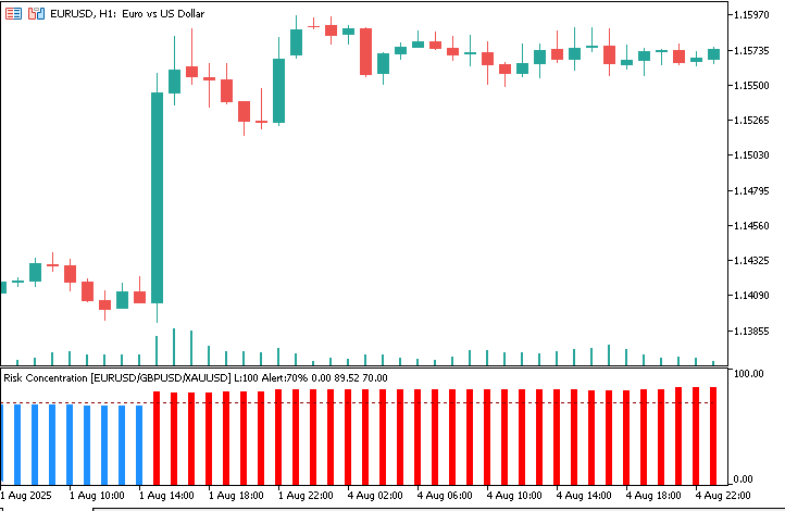
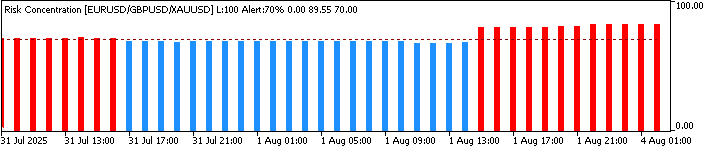
The behavior described in this article can be reproduced with the following configuration. Symbol1, Symbol2 and Symbol3 are EURUSD, GBPUSD and XAUUSD, and both the chart timeframe and CalcTimeframe are H1. LookbackBars is 100, AlertLevel is 70, RecalcEveryBars is 1 and MinValidDataFraction is 0.70. The quotes come from the MetaQuotes-Demo server, using symbol names without suffixes, with H1 history downloaded for all three symbols before the indicator is attached. The figures in this article show the period from 31 July to 4 August 2025 (Figure 1 starts on 1 August), with times given in the chart’s server time.
On this setup, the first 99 bars (LookbackBars − 1) are empty, because no full window exists yet. From the 100th bar onward, the histogram appears on the fixed 0–100 scale, blue below 70 and red at or above it, with the dotted alert line drawn at 70. The sub-window title reads Risk Concentration [EURUSD/GBPUSD/XAUUSD] L:100 Alert:70%.
Over the period shown, the readings stay in a narrow band, from about 68% to roughly 90%. The values quoted here are approximate, read from the figures. On 31 July the bars start just above the alert line, then sit just below it for the rest of that day and into the morning of 1 August. From the early afternoon of 1 August, every bar is red, and the readings climb to the high 80s by 4 August. Figure 1 shows the same move on the EURUSD H1 chart, where the shift to red bars coincides with a large bullish EURUSD candle. Attaching the indicator to a chart whose timeframe differs from CalcTimeframe fails at load with the message described earlier.
Reading the Indicator in Practice
Blue bars mean the dominant eigenvalue accounts for less than the AlertLevel threshold (70% by default) of total portfolio variance; red bars mean it has crossed that threshold. What crossing the threshold tells you is narrower than it might sound: it says the selected numerical level has been exceeded, nothing more. It's tempting to read a red bar as proof that the three instruments have become less independent, but a large eigenvalue share can also come from one instrument simply being far more volatile than the other two, with no real change in how closely they move together. A red bar is best read as a signal to look at the correlations and volatilities behind the number, not as a self-contained verdict that the instruments are now moving as one.
The height of each bar gives the concentration percentage. A bar at 85% means the dominant eigenvalue accounts for 85% of total variance. A bar at 55% means the largest principal direction accounts for 55%, so the variance is less concentrated than at 85%. One qualification: when RecalcEveryBars is greater than 1, not every bar's height comes from a fresh calculation at that bar — most are carried forward from the last bar where the eigendecomposition actually ran, as covered earlier. The plotted height is still the best available estimate of concentration at that point, just not always freshly computed for that exact bar.
What changes the reading over time is the evolving covariance structure of the instruments. During periods of strong macro directionality, such as a sustained dollar trend, a commodity supply shock, or a central bank policy divergence, instruments may become more correlated. As more of their variation moves in the same direction, the dominant eigenvalue can account for a larger share of total variance and the bars may move into the alert region.
The LookbackBars input controls how responsive the indicator is to regime changes. A shorter lookback (say 50 bars) reacts quickly to correlation shifts but is noisier. A longer lookback (200 bars) is smoother but slower to detect new concentration episodes. The default of 100 bars on H1 covers roughly four trading days of hourly observations. This provides a short-term window that still smooths out single-bar noise.
The defaults of 70% for AlertLevel and 0.70 for MinValidDataFraction are illustrative settings, not values derived from optimization, backtesting or a statistical test. They are starting points to calibrate against your own instruments, timeframe and data source.
One way to build intuition for AlertLevel is to translate it into an equivalent correlation. For three series with equal variance and the same pairwise correlation ρ, the dominant eigenvalue’s share of total variance is (1 + 2ρ) / 3:
| AlertLevel | Equivalent ρ (equal variances, equal correlations) |
|---|---|
| 50% | 0.25 |
| 70% | 0.55 |
| 80% | 0.70 |
| 90% | 0.85 |
This is a stylized reference, not a rule. Real baskets have unequal volatilities, and a basket that pairs gold with two currency pairs can show a high share with little correlation at all. A practical way to calibrate is to run the indicator over your own history at several AlertLevel settings and check what fraction of bars turns red, then choose the level that flags the share of history you consider unusual.
MinValidDataFraction works on a simpler principle: how much of the window must hold valid data from all three symbols. With LookbackBars at 100, the settings translate as follows:
| MinValidDataFraction | Valid bars required (of 100) |
|---|---|
| 0.50 | 50 |
| 0.70 | 70 |
| 0.90 | 90 |
| 1.00 | 100 |
A lower fraction keeps the indicator computing through gaps but on smaller samples. A higher fraction gives better-supported readings but leaves more bars empty or carried forward. How gappy your symbols are decides the right trade-off, so treat 0.70 as a place to start rather than a recommendation.
Conclusion
Parts 1 through Part 4 of this series built the analytical toolkit for measuring portfolio risk decomposition — covariance matrices, eigenvalue decomposition, spectral theorem verification, and entropy scoring. Part 5 takes that toolkit and makes it live.
RiskConcentrationIndicator.mq5 introduces three design patterns that will appear in the remaining parts of this series. The rolling prefix sum engine allows the covariance statistics for a lookback window to be recovered in O(1) time with respect to the window length, avoiding a full rescan of the window for each calculation, though extending those sums by one new bar still costs a data lookup per symbol. The timestamp-based alignment via iBarShift() matches each symbol using the chart bar’s timestamp and requires an exact match on the open time of both bars that form the return, so a neighboring bar is never mistaken for a genuine one and a return is never stretched over a missing bar. The indicator is supported only when CalcTimeframe equals the chart’s timeframe. And the principled missing data handling — excluding bars rather than zero-filling them, tracking valid counts separately, refusing to compute below a minimum data fraction — helps prevent the indicator from producing misleading readings when some observations are unavailable, though a stale carried-forward value can still remain on screen through a stretch of missing data.
The histogram uses blue below the threshold and red at or above it. It answers a narrow question: has the covariance structure crossed the chosen numerical threshold at this point? It is not a verdict on whether the portfolio is truly diversified or dominated by a single correlation-driven factor.
Attached File: RiskConcentrationIndicator.mq5
Next: Part 6 — Principal Portfolio Weights: Trading the Eigenvectors
Warning: All rights to these materials are reserved by MetaQuotes Ltd. Copying or reprinting of these materials in whole or in part is prohibited.
This article was written by a user of the site and reflects their personal views. MetaQuotes Ltd is not responsible for the accuracy of the information presented, nor for any consequences resulting from the use of the solutions, strategies or recommendations described.