

Confident Learning: Finding Mislabeled Trades Before They Poison Your Classifier
 106
 0

Introduction
Every meta-labeling system I've built runs on the same quiet assumption: the label I hand the training set is correct. A candidate signal fired, price moved a certain way over the next N bars, so I call it a win or a loss and feed that pair to a classifier. Nobody stops to check whether the label itself deserves to be there.
It usually doesn't, not entirely. A "win" that only cleared the profit threshold because of a single favorable tick, a "loss" that would have been a win if the exit rule looked five bars further - these aren't edge cases, they're baked into how any mechanical labeling heuristic works. The classifier doesn't know the difference between a clean signal and a coin-flip that happened to land right. It just learns whatever pattern the noisy labels contain, confidently.
The uncomfortable part is that this failure mode is invisible to the usual diagnostics. A meta-filter trained on 50% noisy labels won't throw an error or show unusually high training loss. It may still report plausible accuracy on a held-out set, because that set was labeled with the same noisy heuristic. To see the problem, you have to ask a different question than "does this model fit the data?" Ask instead: "which specific rows are likely mislabeled?" That requires a different kind of audit than a standard train/test split.
That's the gap confident learning fills. It doesn't touch the strategy logic, the entry signal, or the exit rule - it sits between "I have a labeled dataset" and "I train a classifier on it," and its only job is to flag rows where the label probably doesn't match what actually happened. Whether removing those rows helps is a separate, empirical question, and that's the part of this article I was the least prepared for.
This article is about auditing that noise before training, not about a new entry signal. The base strategy here (an RSI/trend crossover) is deliberately simple - it exists to generate a labeled dataset with real, uncurated noise in it. The actual subject is CConfidentLabelAuditor: a native MQL5 implementation of confident learning (Northcutt, Athalye, and Mueller, 2021) that estimates which training labels are probably wrong and removes them before the meta-filter is trained on them.
I built an Expert Advisor with a single input flag, InpUseCleanedLabels. It switches meta-filter training between raw labels and the audited (cleaned) subset, while keeping all other inputs identical. That gives a real A/B comparison in the Strategy Tester instead of a claim. I ran it four times: once on raw labels, and three times on cleaned labels at different pruning aggressiveness levels. The results didn't confirm my hunch on the first try, and the honest version of that story is what this article is about.
Where Meta-Label Noise Actually Comes From
The candidate signal itself is a plain RSI/trend crossover - I kept it deliberately unremarkable, since the point of this article is the audit, not the entry rule. A long candidate fires when RSI crosses up through 50 while price sits above its trend SMA; a short candidate mirrors that on the way down:
DetectCandidateSignal
//+------------------------------------------------------------------+
//| DetectCandidateSignal                                            |
//+------------------------------------------------------------------+
//| +1 = long candidate (RSI crosses above 50 while price trends up),|
//| -1 = short candidate (mirror image), 0 = no candidate at shift.  |
//+------------------------------------------------------------------+
int DetectCandidateSignal(const int shift,const double &close[],const double &sma[],
                           const double &rsi[])
  {
   if(rsi[shift] >= 50.0 && rsi[shift + 1] < 50.0 && close[shift] > sma[shift])
      return(1);
   if(rsi[shift] <= 50.0 && rsi[shift + 1] > 50.0 && close[shift] < sma[shift])
      return(-1);
   return(0);
  }
Every candidate gets a four-number feature vector. Three of the four - RSI trigger strength, distance from trend, and recent momentum - are direction-sign-flipped so long and short candidates share one model instead of needing two. The fourth, the ATR ratio, is a non-directional volatility-regime read and is deliberately left unflipped:
ComputeFeatures
//+------------------------------------------------------------------+
//| ComputeFeatures                                                  |
//+------------------------------------------------------------------+
//| All four features are computed strictly from data available AT   |
//| the signal bar - nothing here ever looks past shift. Direction   |
//| (dir) sign-flips the direction-sensitive features so one filter  |
//| can be trained on both long and short candidates together.       |
//+------------------------------------------------------------------+
void ComputeFeatures(const int shift,const int dir,const double &close[],const double &sma[],
                      const double &atr[],const double &atr_long[],const double &rsi[],
                      double &f[])
  {
   double atr_now = MathMax(atr[shift],CL_EPS);

   f[0] = dir * (rsi[shift] - 50.0) / 50.0;                                 // RSI trigger strength
   f[1] = dir * (close[shift] - sma[shift]) / atr_now;                      // distance from trend, in ATRs
   f[2] = atr[shift] / MathMax(atr_long[shift],CL_EPS);                     // volatility-regime ratio
   f[3] = dir * (close[shift] - close[shift + InpMomentumBars]) / atr_now;  // recent momentum
  }
And here's the label heuristic itself - the actual source of the noise this whole article is about.
ComputeLabel
//+------------------------------------------------------------------+
//| ComputeLabel                                                     |
//+------------------------------------------------------------------+
//| ComputeLabel - the (noisy) meta-label: did price move far enough |
//| in the signal's favor, within InpLabelHorizonBars bars, to clear |
//| InpMinNetMovePoints? This ignores the intrabar path and any      |
//| stop-out that would have happened first - exactly the kind of    |
//| shortcut that seeds label noise, and the reason this EA needs    |
//| the auditor in the first place.                                  |
//+------------------------------------------------------------------+
int ComputeLabel(const int shift,const int dir,const double &close[])
  {
   int forward_shift = shift - InpLabelHorizonBars;
   double raw_move_points = dir * (close[forward_shift] - close[shift]) / _Point;
   return(raw_move_points > InpMinNetMovePoints ? 1 : 0);
  }
That single comparison is the entire label. It looks at the close price twenty bars later, checks whether it moved far enough in the signal's favor, and ignores everything in between. A trade that would have been stopped out on bar 3 still reads as a win if price is higher again by bar 20. A trade that was comfortably profitable for fifteen bars still reads as a loss if it gives it all back by bar 20. None of that is a coding mistake - it's what any fixed-horizon forward-return label does, and it's precisely the kind of systematic, structural noise confident learning is built to catch.
The technique doesn't need to know why a label might be wrong. It only needs a classifier that can be cross-validated out-of-fold, and it uses that classifier's own disagreement with the given label - measured honestly, on data the classifier never trained on - as the noise signal.
The Confident Learning Math
The pipeline has five steps, and each one maps to a method on CConfidentLabelAuditor that I'll show in full later. Here's the reasoning behind each step first, since the code is easier to read once the "why" is in place.
1. Out-of-fold probabilities. I split the candidate set into k contiguous time blocks (five by default). For each block, I train a fresh logistic regression on the other k-1 blocks and predict on the held-out block. Every sample ends up with a predicted probability from a model that never saw its label during training - that's what makes the next steps trustworthy instead of circular.
Self-confidence for a sample with given label y and out-of-fold probability p₁ (probability of class 1):
self_confidence = p₁ if y = 1, else (1 - p₁)
Per-class threshold (averaged self-confidence a class needs to "confidently" claim a sample):
t_c = mean of self_confidence over every sample whose given (noisy) label is c - grouped by the label being audited, not by what the model currently guesses
2. Per-class thresholds. Rather than one global cutoff, each class gets its own threshold, computed as the class's own average predicted probability. This is the part of confident learning that lets one class's label noise run hotter than the other's, instead of forcing a single arbitrary cutoff onto both.
3. The confident joint. For every sample, I check which class's threshold it clears. If both clear, the larger margin above threshold wins the tie. If neither clears, the model has no confident opinion and the sample doesn't vote. Every sample that does vote increments a 2x2 count: confident_joint[given_label][confidently_predicted_label]. The off-diagonal cells are the interesting ones - they're candidate mislabels.
4. Calibration. The confident joint's rows won't sum to the real number of examples in each class, because the thresholds don't clear on every sample. I rescale each row so it matches the true label counts - this is what corrects for one class's threshold being systematically stricter than the other's.
5. Rank and prune. For each off-diagonal cell, I take the calibrated count as the estimated number of true mislabels in that cell, and prune exactly that many samples - the ones with the worst self-confidence first. This mirrors cleanlab's prune_counts approach: prune per-cell by rank, not one flat percentile cut across the whole dataset.
Worth being precise about what "worst self-confidence" means here, since it's the number that actually decides which rows get removed. If a candidate was given label 1 (a "win") but the out-of-fold model only assigns it a 0.05 probability of being a win, its self-confidence is 0.05 - about as strong a disagreement as the model can register. A candidate given label 1 that the model scores at 0.48 is a much weaker disagreement, close to a coin flip, and survives longer in the ranking. The auditor always removes the most confidently-contradicted rows first within each cell, which is what keeps the borderline, ambiguous cases in the training set even under aggressive pruning - it's only the clear-cut mislabels that get cut first.
One more distinction matters. Self-confidence measures how strongly the model supports the given label, on a 0–1 scale - the pruning ranking uses this number, and it's also what the FlagView indicator plots later in this article. Normalized margin measures how much the model prefers the given label over the alternative, on a −1–1 scale. The auditor computes and logs normalized margin to the CSV for anyone who wants to inspect it, but the pruning uses self-confidence only.
System Architecture
Three files, one shared library:
ConfidentLearningLib.mqh - CLogRegClassifier (the base learner) and CConfidentLabelAuditor (the five-step pipeline above), plus the SConfidentLearningReport struct the audit returns.
ConfidentLearning_Audit_EA.mq5 - builds a labeled candidate set from an RSI/trend crossover signal every InpRefitEveryBars bars, runs the audit, trains the live meta-filter on either the raw or cleaned set depending on InpUseCleanedLabels, and trades whatever that filter approves above InpProbThreshold. Every refit writes two audit CSV logs.
ConfidentLearning_FlagView.mq5 - a separate-window indicator that reads the EA's audit log and plots each audited signal's self-confidence, marking the ones the auditor pruned.
The feature vector is the four numbers shown in the next section: RSI trigger strength, distance from the trend SMA in ATR units, a fast/slow ATR ratio for the volatility regime, and recent momentum - all direction-sign-flipped so long and short candidates train one shared model. The base learner is a small logistic regression trained by batch gradient descent with L2 regularization, used both inside the auditor's cross-fitting and as the final filter the EA actually trades with. Keeping both on the same simple model isolates the effect of label cleaning from any effect of model complexity - if I'd used a bigger model for the final filter than for the fold models, any difference between the raw and cleaned runs could just as easily be attributed to that mismatch instead of to the cleaning itself.
Every refit cycle runs the same six steps in order: scan the last InpTrainWindowBars bars for candidate signals, compute features and labels for each one, hand the resulting dataset to CConfidentLabelAuditor::Audit, branch on InpUseCleanedLabels to decide which rows the final model actually trains on, retrain g_final_model, and write both CSV logs. That cycle repeats every InpRefitEveryBars bars for the life of the backtest - the model isn't static, it's re-audited and refit on a rolling basis as new bars close.
The Base Learner: CLogRegClassifier
Nothing exotic here - a textbook logistic regression, chosen deliberately small so any performance difference between runs comes from the training data, not from a more expressive model finding structure in the noise.
SConfidentLearningReport struct and CLogRegClassifier declaration
//+------------------------------------------------------------------+
//| SConfidentLearningReport struct                                  |
//+------------------------------------------------------------------+
struct SConfidentLearningReport
  {
   int    n_total;                   // candidate signals audited in this refit window
   int    n_flagged;                 // samples pruned as likely-mislabeled, at the run's
                                      // InpPruneAggressiveness setting
   double est_noise_rate;            // aggressiveness-INDEPENDENT estimate: the calibrated
                                      // joint's off-diagonal mass over n - how much of the
                                      // dataset the auditor believes is mislabeled, before
                                      // any pruning policy is applied to it
   double prune_rate;                // n_flagged / n - how much was ACTUALLY pruned this run,
                                      // which moves with InpPruneAggressiveness and is NOT
                                      // the same number as est_noise_rate except at
                                      // aggressiveness 1.0
   double calibrated_joint[][2];     // calibrated_joint[given_label][confident_label] counts
                                      // (dynamic outer dim - MQL5 requires that for a struct
                                      // member that gets passed by reference into a function)
  };

//+------------------------------------------------------------------+
//| CLogRegClassifier class                                          |
//+------------------------------------------------------------------+
class CLogRegClassifier
  {
private:
   double            m_weights[];    // one weight per feature, set by Train()
   double            m_bias;         // intercept term
   int               m_num_features; // feature vector length this instance expects
   bool              m_ready;        // true once Train() has produced usable weights

public:
                     CLogRegClassifier(void);
   void              Init(const int num_features);
   double            Sigmoid(const double z);
   bool              Train(const double &features[][CL_NUM_FEATURES],const int &labels[],
                            const int n_samples,const int epochs,const double learning_rate,
                            const double l2);
   double            PredictProba(const double &feature_row[]);
   bool              IsReady(void) const { return(m_ready); }
  };
The training loop is plain batch gradient descent on the logistic loss, with L2 applied only to the weights (never the bias, so the intercept stays free to track the base rate of whatever window it's trained on):
CLogRegClassifier::Train
//+------------------------------------------------------------------+
//| CLogRegClassifier::Train                                         |
//+------------------------------------------------------------------+
bool CLogRegClassifier::Train(const double &features[][CL_NUM_FEATURES],const int &labels[],
                               const int n_samples,const int epochs,const double learning_rate,
                               const double l2)
  {
//--- refuse to fit a line through fewer points than the model has
//--- degrees of freedom - a silently-wrong model is worse than none
   if(n_samples < m_num_features + 2)
      return(false);

   ArrayInitialize(m_weights,0.0);
   m_bias = 0.0;

   double grad_w[];
   ArrayResize(grad_w,m_num_features);

   for(int epoch = 0; epoch < epochs; epoch++)
     {
      ArrayInitialize(grad_w,0.0);
      double grad_b = 0.0;

      for(int i = 0; i < n_samples; i++)
        {
         double z = m_bias;
         for(int j = 0; j < m_num_features; j++)
            z += m_weights[j] * features[i][j];
         double p   = Sigmoid(z);
         double err = p - labels[i];         // logistic loss gradient w.r.t. the logit
         for(int j = 0; j < m_num_features; j++)
            grad_w[j] += err * features[i][j];
         grad_b += err;
        }

      //--- average over the batch, then add the L2 penalty on the weights
      //--- only (never on the bias, so the intercept stays free to match
      //--- the base rate of the training window)
      for(int j = 0; j < m_num_features; j++)
        {
         grad_w[j] = grad_w[j] / n_samples + l2 * m_weights[j];
         m_weights[j] -= learning_rate * grad_w[j];
        }
      grad_b /= n_samples;
      m_bias -= learning_rate * grad_b;
     }

   m_ready = true;
   return(true);
  }
That first guard - n_samples < m_num_features + 2 - matters more than it looks. It comes back later in this article, because it's the actual mechanical reason aggressive pruning backfired in my results.
Train calls Sigmoid internally, and BuildOutOfFold (next section) calls Init and PredictProba on each fold's model - all three are short enough to show together instead of scattering them:
CLogRegClassifier::Init, Sigmoid, PredictProba
//+------------------------------------------------------------------+
//| CLogRegClassifier::Init, Sigmoid, PredictProba                   |
//+------------------------------------------------------------------+
void CLogRegClassifier::Init(const int num_features)
  {
   m_num_features = num_features;
   m_bias         = 0.0;
   m_ready        = false;
   ArrayResize(m_weights,num_features);
   ArrayInitialize(m_weights,0.0);
  }

double CLogRegClassifier::Sigmoid(const double z)
  {
//--- clamp the exponent so MathExp never overflows on a stray large
//--- logit - the saturated 0.0/1.0 output is the mathematically
//--- correct limit anyway
   if(z < -40.0)
      return(0.0);
   if(z > 40.0)
      return(1.0);
   return(1.0 / (1.0 + MathExp(-z)));
  }

double CLogRegClassifier::PredictProba(const double &feature_row[])
  {
   double z = m_bias;
   for(int j = 0; j < m_num_features; j++)
      z += m_weights[j] * feature_row[j];
   return(Sigmoid(z));
  }
Init is what makes the k-fold cross-fitting in BuildOutOfFold honest - each fold gets a model reset to zero weights, so no fold's out-of-fold prediction ever leaks information from the training rows it was scored against. Sigmoid clamps its input before exponentiating for the same reason most people learn to do this the hard way: an unclamped logistic on a stray large logit overflows MathExp and hands you a NaN that quietly poisons everything downstream.
The Auditor: CConfidentLabelAuditor
This class is the article. Every method below maps directly to one of the five steps from the math section, pulled verbatim from the same source file that shipped in the archive - nothing here is retyped or paraphrased.
CConfidentLabelAuditor::BuildOutOfFold
//+------------------------------------------------------------------+
//| CConfidentLabelAuditor::BuildOutOfFold                           |
//+------------------------------------------------------------------+
void CConfidentLabelAuditor::BuildOutOfFold(const double &features[][CL_NUM_FEATURES],
                                             const int &labels[],const int n,const int epochs,
                                             const double learning_rate,const double l2,
                                             double &oof_probs[])
  {
   ArrayResize(oof_probs,n);
   ArrayInitialize(oof_probs,0.5);   // neutral fallback for any row a fold never covers

   for(int fold = 0; fold < m_k_folds; fold++)
     {
      //--- contiguous-block fold assignment (not a random shuffle): keeping
      //--- each fold as one time-ordered block, rather than interleaving
      //--- individual bars, limits how much adjacent, autocorrelated bars
      //--- leak between a fold's train and held-out sides
      int held_out_count = 0;
      for(int i = 0; i < n; i++)
         if((i * m_k_folds) / n == fold)
            held_out_count++;
      if(held_out_count == 0 || held_out_count == n)
         continue;

      double train_features[][CL_NUM_FEATURES];
      int    train_labels[];
      ArrayResize(train_features,n - held_out_count);
      ArrayResize(train_labels,n - held_out_count);

      int t = 0;
      for(int i = 0; i < n; i++)
        {
         if((i * m_k_folds) / n == fold)
            continue;
         for(int j = 0; j < m_num_features; j++)
            train_features[t][j] = features[i][j];
         train_labels[t] = labels[i];
         t++;
        }

      CLogRegClassifier fold_model;
      fold_model.Init(m_num_features);
      if(!fold_model.Train(train_features,train_labels,t,epochs,learning_rate,l2))
         continue;

      double row[];
      ArrayResize(row,m_num_features);
      for(int i = 0; i < n; i++)
        {
         if((i * m_k_folds) / n != fold)
            continue;
         for(int j = 0; j < m_num_features; j++)
            row[j] = features[i][j];
         oof_probs[i] = fold_model.PredictProba(row);
        }
     }
  }
CConfidentLabelAuditor::ComputeThresholds and BuildConfidentJoint
//+------------------------------------------------------------------+
//| CConfidentLabelAuditor::ComputeThresholds                        |
//+------------------------------------------------------------------+
void CConfidentLabelAuditor::ComputeThresholds(const double &oof_probs[],const int &labels[],
                                                const int n,double &t0,double &t1)
  {
   double sum0 = 0.0, sum1 = 0.0;
   int    n0 = 0, n1 = 0;

   for(int i = 0; i < n; i++)
     {
      if(labels[i] == 1)
        {
         sum1 += oof_probs[i];
         n1++;
        }
      else
        {
         sum0 += (1.0 - oof_probs[i]);
         n0++;
        }
     }

//--- each class thresholds itself off its own average predicted
//--- probability - this is what lets one class's noise level differ
//--- from the other's instead of sharing a single arbitrary cutoff
   t1 = (n1 > 0 ? sum1 / n1 : 0.5);
   t0 = (n0 > 0 ? sum0 / n0 : 0.5);
  }

//+------------------------------------------------------------------+
//| CConfidentLabelAuditor::BuildConfidentJoint                      |
//+------------------------------------------------------------------+
void CConfidentLabelAuditor::BuildConfidentJoint(const double &oof_probs[],const int &labels[],
                                                  const int n,const double t0,const double t1,
                                                  int &confident_joint[][2],int &confident_class[])
  {
   ArrayResize(confident_joint,2);        // dynamic outer dim - size it before first use
   confident_joint[0][0] = 0; confident_joint[0][1] = 0;
   confident_joint[1][0] = 0; confident_joint[1][1] = 0;
   ArrayResize(confident_class,n);

   for(int i = 0; i < n; i++)
     {
      double p1 = oof_probs[i];
      double p0 = 1.0 - p1;
      bool   passes0 = (p0 >= t0);
      bool   passes1 = (p1 >= t1);

      if(!passes0 && !passes1)
        {
         //--- neither class clears its own threshold - the model has no
         //--- confident opinion on this sample, so it cannot vote either way
         confident_class[i] = -1;
         continue;
        }

      if(passes0 && passes1)
        {
         //--- both clear - break the tie toward whichever class the model is
         //--- confident in by the larger margin above its own threshold
         confident_class[i] = ((p1 - t1) > (p0 - t0) ? 1 : 0);
        }
      else
        {
         confident_class[i] = (passes1 ? 1 : 0);
        }

      confident_joint[labels[i]][confident_class[i]]++;
     }
  }
Calibration rescales each row of that joint against the real per-class counts, so a stricter threshold on one class doesn't make it look artificially cleaner than the other:
CConfidentLabelAuditor::CalibrateJoint
//+------------------------------------------------------------------+
//| CConfidentLabelAuditor::CalibrateJoint                           |
//+------------------------------------------------------------------+
void CConfidentLabelAuditor::CalibrateJoint(const int &confident_joint[][2],const int &labels[],
                                             const int n,double &calibrated_joint[][2])
  {
   ArrayResize(calibrated_joint,2);       // dynamic outer dim - size it before first use
   int row_sum[2];
   row_sum[0] = confident_joint[0][0] + confident_joint[0][1];
   row_sum[1] = confident_joint[1][0] + confident_joint[1][1];

   int label_count[2] = {0, 0};
   for(int i = 0; i < n; i++)
      label_count[labels[i]]++;

//--- rescale each row so it sums to the ACTUAL number of examples
//--- given that label, not to however many the thresholds happened
//--- to rule confidently on - this is what corrects for one class's
//--- threshold being stricter than the other's
   for(int i = 0; i < 2; i++)
     {
      for(int j = 0; j < 2; j++)
        {
         if(row_sum[i] > 0)
            calibrated_joint[i][j] = (double)confident_joint[i][j] *
                                      ((double)label_count[i] / (double)row_sum[i]);
         else
            calibrated_joint[i][j] = 0.0;
        }
     }
  }
RankAndFlag leans on two small private helpers for the two numbers it logs per sample - shown here since they're called, not just described:
CConfidentLabelAuditor::SelfConfidence and NormalizedMargin
//+------------------------------------------------------------------+
//| CConfidentLabelAuditor::SelfConfidence                           |
//+------------------------------------------------------------------+
double CConfidentLabelAuditor::SelfConfidence(const double p1,const int given_label)
  {
//--- probability the model out-of-fold assigns to the label the
//--- sample was actually GIVEN - low means the model confidently
//--- disagrees with the trainer's own label
   return(given_label == 1 ? p1 : 1.0 - p1);
  }

//+------------------------------------------------------------------+
//| CConfidentLabelAuditor::NormalizedMargin                         |
//+------------------------------------------------------------------+
double CConfidentLabelAuditor::NormalizedMargin(const double p1,const int given_label)
  {
   double p_given = (given_label == 1 ? p1 : 1.0 - p1);
   double p_other = (given_label == 1 ? 1.0 - p1 : p1);
   return(p_given - p_other);
  }
And the actual pruning - worst self-confidence first, per off-diagonal cell, up to that cell's calibrated count:
CConfidentLabelAuditor::RankAndFlag
//+------------------------------------------------------------------+
//| CConfidentLabelAuditor::RankAndFlag                              |
//+------------------------------------------------------------------+
void CConfidentLabelAuditor::RankAndFlag(const double &oof_probs[],const int &labels[],
                                          const int &confident_class[],const int n,
                                          const double &calibrated_joint[][2],bool &is_flagged[],
                                          double &self_conf[],double &norm_margin[])
  {
   ArrayResize(is_flagged,n);
   ArrayResize(self_conf,n);
   ArrayResize(norm_margin,n);
   for(int i = 0; i < n; i++)
     {
      is_flagged[i]  = false;
      self_conf[i]   = SelfConfidence(oof_probs[i],labels[i]);
      norm_margin[i] = NormalizedMargin(oof_probs[i],labels[i]);
     }

//--- prune each off-diagonal cell independently, worst self-confidence
//--- first, up to the calibrated count for that cell - this mirrors
//--- cleanlab's prune_counts approach instead of one flat percentile
//--- cut across the whole dataset
   for(int given = 0; given < 2; given++)
     {
      for(int predicted = 0; predicted < 2; predicted++)
        {
         if(given == predicted)
            continue;

         int target = (int)MathRound(m_prune_aggressiveness * calibrated_joint[given][predicted]);
         if(target <= 0)
            continue;

         int    cell_indices[];
         int    cell_n = 0;
         ArrayResize(cell_indices,n);
         for(int i = 0; i < n; i++)
            if(labels[i] == given && confident_class[i] == predicted)
               cell_indices[cell_n++] = i;
         ArrayResize(cell_indices,cell_n);

         //--- simple insertion sort by ascending self-confidence - cell sizes
         //--- are small (bounded by the estimated noise count), so O(n^2) here
         //--- never matters in practice
         for(int a = 1; a < cell_n; a++)
           {
            int    key_idx = cell_indices[a];
            double key_val = self_conf[key_idx];
            int    b = a - 1;
            while(b >= 0 && self_conf[cell_indices[b]] > key_val)
              {
               cell_indices[b + 1] = cell_indices[b];
               b--;
              }
            cell_indices[b + 1] = key_idx;
           }

         int flag_count = MathMin(target,cell_n);
         for(int a = 0; a < flag_count; a++)
            is_flagged[cell_indices[a]] = true;
        }
     }
  }
Once pruning decides which rows are noisy, something has to actually build the cleaned training set the refit uses. That's BuildCleanedDataset - it's called from the EA's RefitPipeline branch shown earlier, so here's the real implementation rather than a description of what it does:
CConfidentLabelAuditor::BuildCleanedDataset
//+------------------------------------------------------------------+
//| CConfidentLabelAuditor::BuildCleanedDataset                      |
//+------------------------------------------------------------------+
void CConfidentLabelAuditor::BuildCleanedDataset(const double &features[][CL_NUM_FEATURES],
                                                  const int &labels[],const bool &is_flagged[],
                                                  const int n,
                                                  double &out_features[][CL_NUM_FEATURES],
                                                  int &out_labels[],int &out_n)
  {
   int kept = 0;
   for(int i = 0; i < n; i++)
      if(!is_flagged[i])
         kept++;

   ArrayResize(out_features,kept);
   ArrayResize(out_labels,kept);

   int t = 0;
   for(int i = 0; i < n; i++)
     {
      if(is_flagged[i])
         continue;
      for(int j = 0; j < m_num_features; j++)
         out_features[t][j] = features[i][j];
      out_labels[t] = labels[i];
      t++;
     }
   out_n = kept;
  }
It's a plain filter - keep the row if it wasn't flagged, skip it if it was, and hand back a fresh array sized to whatever actually survived the prune. Nothing more complicated than that, which is the point: the auditor's job stops at deciding what to keep.
And the orchestration method that ties all five steps together into one call the EA makes on every refit:
CConfidentLabelAuditor::Audit
//+------------------------------------------------------------------+
//| CConfidentLabelAuditor::Audit                                    |
//+------------------------------------------------------------------+
SConfidentLearningReport CConfidentLabelAuditor::Audit(const double &features[][CL_NUM_FEATURES],
                                                        const int &labels[],const int n,
                                                        const int epochs,
                                                        const double learning_rate,const double l2,
                                                        bool &is_flagged[],double &self_conf[],
                                                        double &norm_margin[])
  {
   SConfidentLearningReport report;
   double oof_probs[];
   int    confident_joint[][2];
   int    confident_class[];
   double t0, t1;

   BuildOutOfFold(features,labels,n,epochs,learning_rate,l2,oof_probs);
   ComputeThresholds(oof_probs,labels,n,t0,t1);
   BuildConfidentJoint(oof_probs,labels,n,t0,t1,confident_joint,confident_class);
   CalibrateJoint(confident_joint,labels,n,report.calibrated_joint);

   //--- the aggressiveness-independent estimate has to be read off the
   //--- calibrated joint BEFORE RankAndFlag applies m_prune_aggressiveness -
   //--- RankAndFlag's own flagged count is already downstream of that
   //--- multiplier and cannot be used to answer "how much noise did the
   //--- auditor estimate", only "how much did this run's policy prune"
   report.est_noise_rate = (n > 0 ?
      (report.calibrated_joint[0][1] + report.calibrated_joint[1][0]) / (double)n : 0.0);

   RankAndFlag(oof_probs,labels,confident_class,n,report.calibrated_joint,is_flagged,
               self_conf,norm_margin);

   report.n_total = n;
   int flagged = 0;
   for(int i = 0; i < n; i++)
      if(is_flagged[i])
         flagged++;
   report.n_flagged  = flagged;
   report.prune_rate = (n > 0 ? (double)flagged / (double)n : 0.0);

   return(report);
  }
The EA: Toggling Raw vs. Cleaned Training
The whole A/B comparison hinges on one input and one branch. Everything upstream of this - feature computation, the label heuristic, the audit itself - runs identically regardless of which way the flag is set:
Confident Learning input group
input group                "=== Confident Learning ===";
input int      InpTrainWindowBars   = 3000;    // history scanned for candidate signals per refit
input int      InpRefitEveryBars    = 250;     // bars between audit + retrain cycles
input int      InpMinTrainSamples   = 60;      // skip the audit below this many candidates
input int      InpKFolds            = 5;       // cross-fitting folds for out-of-fold probabilities
input double   InpPruneAggressiveness = 1.0;   // 0..1 multiplier on the estimated noise counts
input bool     InpUseCleanedLabels  = true;    // false = train the filter on the raw labels
input int      InpCLEpochs          = 300;     // gradient-descent epochs (fold and final models)
input double   InpCLLearningRate    = 0.10;    // gradient-descent learning rate
input double   InpCLL2              = 0.001;   // L2 regularization strength
And the branch inside RefitPipeline() that actually uses it, right after the audit has run:
RefitPipeline - raw vs. cleaned training set selection
   bool   is_flagged[];
   double self_conf[];
   double norm_margin[];
   g_last_report = g_auditor.Audit(features,labels,n,InpCLEpochs,InpCLLearningRate,InpCLL2,
                                    is_flagged,self_conf,norm_margin);

   double train_features[][CL_NUM_FEATURES];
   int    train_labels[];
   int    train_n;

   if(InpUseCleanedLabels)
     {
      g_auditor.BuildCleanedDataset(features,labels,is_flagged,n,train_features,train_labels,
                                     train_n);
     }
   else
     {
      ArrayResize(train_features,n);
      ArrayResize(train_labels,n);
      for(int i = 0; i < n; i++)
        {
         for(int j = 0; j < CL_NUM_FEATURES; j++)
            train_features[i][j] = features[i][j];
         train_labels[i] = labels[i];
        }
      train_n = n;
     }

   bool train_ok = g_final_model.Train(train_features,train_labels,train_n,InpCLEpochs,
                                        InpCLLearningRate,InpCLL2);
if(!train_ok)
   PrintFormat("ConfidentLearning_Audit_EA: Train() failed (train_n=%d, needs >= %d) - "
               "keeping the last successfully trained model",train_n,CL_NUM_FEATURES + 2);
Notice the audit itself - g_auditor.Audit(...) - always runs, in both branches. InpUseCleanedLabels only controls whether is_flagged is actually used to filter the training rows. That's a deliberate design choice: the printed audit stats (n_total, n_flagged, est_noise_rate) are always available for logging, even on a raw-label run, without changing what that run actually trades on. It also means a raw-labels run and a cleaned-labels run at the same InpPruneAggressiveness always report identical audit numbers in the Journal - which is exactly what I saw across my own runs, and a useful sanity check that the branch is wired correctly rather than silently changing what gets audited.
The other input that matters here is InpMinTrainSamples. If a given refit window doesn't produce at least this many candidates, the whole refit is skipped for that cycle rather than forcing a fit on too little data - the same "refuse rather than fit badly" philosophy as the guard inside CLogRegClassifier::Train from the previous section.
The EA: Risk and Order Management
This section is not specific to confident learning - it's the standing order-management discipline I apply to every EA I publish. It matters here because changes in approval rate change how often the order-management path is exercised. The aggressiveness-1.0 run approved 71 trades against the raw run's 24, and every one of those extra 47 trades still had to pass through the same margin, minimum-lot, and stop-distance guards below - a sizing bug that only shows up rarely would have been three times more likely to surface in that run purely from trade-count exposure. The guards below must stay identical across runs to keep the comparison valid. Four guards, in order: clamp by real margin (not just the risk formula), never round a sub-minimum lot up, floor the stop distance by the broker's real minimum before sizing, and clamp to both the per-order limit and the symbol maximum.
ComputeRiskNormalizedLots
//+------------------------------------------------------------------+
//| ComputeRiskNormalizedLots                                        |
//+------------------------------------------------------------------+
double ComputeRiskNormalizedLots(const double sl_distance_price,const bool is_buy)
  {
   double tick_value = SymbolInfoDouble(_Symbol,SYMBOL_TRADE_TICK_VALUE);
   double tick_size  = SymbolInfoDouble(_Symbol,SYMBOL_TRADE_TICK_SIZE);
   if(tick_size <= 0.0 || tick_value <= 0.0)
      return(0.0);                                    // symbol spec is unusable

   double loss_per_lot = (sl_distance_price / tick_size) * tick_value;
   if(loss_per_lot <= 0.0)
      return(0.0);

   double risk_amount = AccountInfoDouble(ACCOUNT_BALANCE) * InpRiskPercent / 100.0;
   double raw_lots     = risk_amount / loss_per_lot;

   double lot_step  = SymbolInfoDouble(_Symbol,SYMBOL_VOLUME_STEP);
   double lot_min   = SymbolInfoDouble(_Symbol,SYMBOL_VOLUME_MIN);
   double lot_max   = SymbolInfoDouble(_Symbol,SYMBOL_VOLUME_MAX);
   double lot_limit = SymbolInfoDouble(_Symbol,SYMBOL_VOLUME_LIMIT);

//--- rounded DOWN, never to nearest: rounding up would quietly risk
//--- more than InpRiskPercent
   double lots = (lot_step > 0.0 ? MathFloor(raw_lots / lot_step) * lot_step : raw_lots);

//--- rule (2): below the broker minimum, skip the trade rather than
//--- force it up to lot_min
   if(lots < lot_min)
      return(0.0);

//--- rule (4): clamp to BOTH the per-order limit and the max, not
//--- the max alone
   if(lot_limit > 0.0)
      lots = MathMin(lots,lot_limit);
   if(lot_max > 0.0)
      lots = MathMin(lots,lot_max);

//--- rule (1): re-clamp by actual free margin, not the risk formula's
//--- assumption that margin is always available
   double price = (is_buy ? SymbolInfoDouble(_Symbol,SYMBOL_ASK) : SymbolInfoDouble(_Symbol,SYMBOL_BID));
   double margin_required = 0.0;
   ENUM_ORDER_TYPE order_type = (is_buy ? ORDER_TYPE_BUY : ORDER_TYPE_SELL);
   if(OrderCalcMargin(order_type,_Symbol,lots,price,margin_required) && margin_required > 0.0)
     {
      double free_margin = AccountInfoDouble(ACCOUNT_MARGIN_FREE);
      if(margin_required > free_margin)
        {
         double scale = free_margin / margin_required;
         lots = (lot_step > 0.0 ? MathFloor((lots * scale) / lot_step) * lot_step : lots * scale);
        }
     }

   if(lots < lot_min)
      return(0.0);                                    // margin clamp pushed it back below minimum
   return(lots);
  }
And the stop-distance floor that runs before sizing, in ExecuteTrade() - the broker's stops/freeze level plus current spread plus a fixed safety pad, so a symbol that reports zero for both still gets a sane minimum distance:
ExecuteTrade - minimum stop distance floor
   double stops_level  = (double)SymbolInfoInteger(_Symbol,SYMBOL_TRADE_STOPS_LEVEL) * _Point;
   double freeze_level = (double)SymbolInfoInteger(_Symbol,SYMBOL_TRADE_FREEZE_LEVEL) * _Point;
   double spread_price = (double)SymbolInfoInteger(_Symbol,SYMBOL_SPREAD) * _Point;

//--- rule (3): floor the stop distance by the broker's real minimum
//--- BEFORE sizing - some symbols report 0 for stops/freeze level, so
//--- the spread + safety pad still applies even then
   double min_stop_distance = MathMax(stops_level,freeze_level) + spread_price +
                               InpStopSafetyPadPoints * _Point;

   double sl_distance = MathMax(InpStopATRMult * atr_value,min_stop_distance);
   double tp_distance = MathMax(InpTakeATRMult * atr_value,min_stop_distance);
The FlagView Indicator
A separate-window indicator with no trading logic of its own - it just reads the audit CSV the EA writes and plots it, so a flagged signal is something you can look at on a chart instead of only reading in a log. Both files share MQL5's common data folder rather than the per-terminal one (FILE_COMMON on every FileOpen call in both the EA and the indicator), specifically so a Strategy Tester run and a live chart on the same machine can read and write the same two CSVs without any extra plumbing.
It loads the file once on init, sorts it by time (MQL5's 2D ArraySort sorts by column 0 while keeping the paired index in column 1 attached to each row - a convenient way to sort-with-carry without a manual struct), then binary-searches it per bar in OnCalculate:
LoadAuditFile - sort-by-time with carried index
//--- sort by time using MQL5's row-preserving 2D ArraySort: column 0
//--- is the sort key, column 1 carries the original row index along
   double sort_key[][2];
   ArrayResize(sort_key,raw_n);
   for(int i = 0; i < raw_n; i++)
     {
      sort_key[i][0] = (double)raw_time[i];
      sort_key[i][1] = (double)i;
     }
   ArraySort(sort_key);
OnCalculate calls one more small helper per bar - BinarySearchTime - which is what makes the per-bar lookup cheap instead of an O(n) scan through the whole audit log on every recalculation:
BinarySearchTime
//+------------------------------------------------------------------+
//| BinarySearchTime                                                 |
//+------------------------------------------------------------------+
int BinarySearchTime(const datetime target)
  {
   int lo = 0, hi = g_audit_n - 1;
   while(lo <= hi)
     {
      int mid = (lo + hi) / 2;
      if(g_audit_time[mid] == target)
         return(mid);
      if(g_audit_time[mid] < target)
         lo = mid + 1;
      else
         hi = mid - 1;
     }
   return(-1);
  }
Standard binary search over the time-sorted array LoadAuditFile built - a hit returns the row index straight away, a miss returns -1 and OnCalculate just leaves that bar's buffers at EMPTY_VALUE. Most bars are misses, since the auditor only logs a row for bars where DetectCandidateSignal actually fired.
OnCalculate - matching audited signals to chart bars
int OnCalculate(const int rates_total,const int prev_calculated,const datetime &time[],
                 const double &open[],const double &high[],const double &low[],
                 const double &close[],const long &tick_volume[],const long &volume[],
                 const int &spread[])
  {
   if(g_audit_n == 0)
      return(rates_total);

//--- recompute only the newly closed bars, same incremental pattern
//--- as every other buffer-based indicator in this project
   int start = (prev_calculated > 1 ? prev_calculated - 1 : 0);

   for(int i = start; i < rates_total; i++)
     {
      BufferSelfConf[i] = EMPTY_VALUE;
      BufferFlagged[i]  = EMPTY_VALUE;

      int idx = BinarySearchTime(time[i]);
      if(idx < 0)
         continue;

      BufferSelfConf[i] = g_audit_self_conf[idx];
      if(g_audit_flagged[idx])
         BufferFlagged[i] = g_audit_self_conf[idx];
     }

   return(rates_total);
  }
On a live EURUSD H1 chart, loaded against the audit log from the aggressiveness-0.25 run, it looks like this - the blue line is self-confidence wherever a candidate signal was audited, and each red marker is a signal the auditor pruned before the final filter ever trained on it:
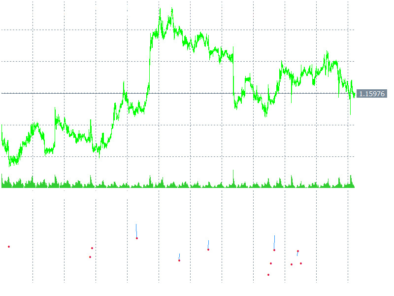
Fig. 1. ConfidentLearning_FlagView on a live EURUSD H1 chart. Red markers are signals the auditor pruned; the blue segments are self-confidence at audited bars.
Testing Setup
Every run below used the same MetaQuotes-Demo account, EURUSD H1, 2026.01.01 to 2026.09.12, deposit 10,000 USD at 1:100 leverage, every-tick modeling on real ticks, zero-latency execution, Optimization disabled (single test pass, not a sweep). History quality reported 99% across all runs, 4,342 bars, 33,247,691 ticks. Every input besides InpUseCleanedLabels and InpPruneAggressiveness stayed fixed at its default: InpRSIPeriod=14, InpTrendSMAPeriod=50, InpATRPeriod=14, InpATRLongPeriod=50, InpLabelHorizonBars=20, InpMinNetMovePoints=60, InpTrainWindowBars=3000, InpRefitEveryBars=250, InpKFolds=5, InpProbThreshold=0.60, InpRiskPercent=1.0, InpMomentumBars=5, InpStopATRMult=2.0, InpTakeATRMult=3.0, InpStopSafetyPadPoints=10. Execution: floating spread (the account's real variable bid/ask spread replayed from tick data, not a fixed point value), and no commission - this demo account's symbol configuration doesn't model one.
Four passes: raw labels, then cleaned labels at three pruning aggressiveness levels (1.0, 0.5, 0.25). Everything else identical across all four - same date range, same symbol, same deposit, same Optimization-disabled single-pass setting. The only thing that changes between the four Strategy Tester runs is the value of two inputs: InpUseCleanedLabels and InpPruneAggressiveness. I picked single test passes over an Optimization Report sweep deliberately here - four clearly-labeled, individually-verifiable runs are easier to audit for honesty than one aggregated report, and this article is explicitly about not taking a pipeline's own numbers at face value.
Results: The Aggressiveness Sensitivity Sweep
The first comparison I ran - raw labels against cleaned labels at full aggressiveness - did not go the way I expected.
| Run | Net profit | Profit factor | Trades | Max equity DD | Sharpe | n_flagged / prune rate | Est. noise rate |
|---|---|---|---|---|---|---|---|
| Raw labels (no cleaning) | -$194.84 | 0.87 | 24 | 7.40% | -1.10 | - | 0.5054 |
| Cleaned, aggressiveness 1.0 | -$762.85 | 0.83 | 71 | 15.67% | -1.57 | 89/0.5028 | 0.5054 |
| Cleaned, aggressiveness 0.5 | -$28.33 | 0.99 | 66 | 9.94% | -0.06 | 45/0.2542 | 0.5054* |
| Cleaned, aggressiveness 0.25 | +$133.63 | 1.04 | 57 | 7.73% | 0.33 | 22/0.1243 | 0.5054 |
*The 0.5 row's noise estimate wasn't pulled from an independent run of that exact setting - it's the same figure the 1.0 and 0.25 reruns both logged, carried over on the strength of the code itself: BuildConfidentJoint and CalibrateJoint never see InpPruneAggressiveness at all, only RankAndFlag does, downstream of calibration. Two independent runs logging the identical calibrated joint is what makes that carry-over something more than an assumption.
This table separates two numbers the first draft conflated. n_flagged / prune rate is n_flagged/n - how much a given run's policy actually removed, which moves with InpPruneAggressiveness. Est. noise rate is the calibrated confident joint's off-diagonal mass over n - the auditor's estimate of how much of the label set is mislabeled, fixed before any pruning policy touches it. I reran the raw and 0.25 passes specifically to log audit_summary.csv's calibrated_joint columns directly rather than leave this number as a gap, and both runs came back at 0.5054 for the final refit window - identical, which is exactly what the code predicts.
At full aggressiveness, the auditor flagged and pruned 89 of 177 candidates - almost exactly matching its independently-measured 0.5054 noise estimate, since at aggressiveness 1.0 the policy acts on nearly everything it believes is mislabeled. Removing all of them before training made the live filter noticeably worse, not better: deeper drawdown, more than triple the trade count, and a lower profit factor than even the untouched raw-label baseline. That's the opposite of the result I went in expecting, and I'm reporting it as it happened rather than reframing it after the fact.
The trade-count jump is the detail that first told me something structural was going on rather than just "the cleaned model is a bit worse." Going from 24 trades on raw labels to 71 on aggressively-cleaned labels isn't a small shift in a filter's selectivity - it's a filter approving roughly three times as many candidate signals above the same 0.60 probability threshold. That only happens if the retrained weights shifted meaningfully, which is consistent with a model fit on a much smaller, higher-variance training set rather than one that simply learned a cleaner version of the same decision boundary.
Softening the pruning tells a cleaner story. At 0.5, the cleaned run pulls back to nearly break-even and above the raw baseline's profit factor, with trade count still elevated at 66 but drawdown roughly half of the aggressiveness-1.0 run. At 0.25, it's the best result of the sweep on every metric: the only profitable run, the lowest drawdown, and the only positive Sharpe ratio - and the trade count (57) and flagged-sample count (22, a 12.4% prune rate) have both settled into a range that looks far more plausible for a labeling heuristic that ignores the intrabar path than the 89-candidate removal at full aggressiveness. Worth being precise about what that 12.4% actually means, though: the underlying noise estimate at this setting is still the same 0.5054 as every other row - 0.25 aggressiveness doesn't mean "the auditor thinks only 12% is noisy," it means the policy is deliberately acting on only the clearest quarter of what it believes is mislabeled, leaving the rest in the training set rather than pruning on the full estimate.
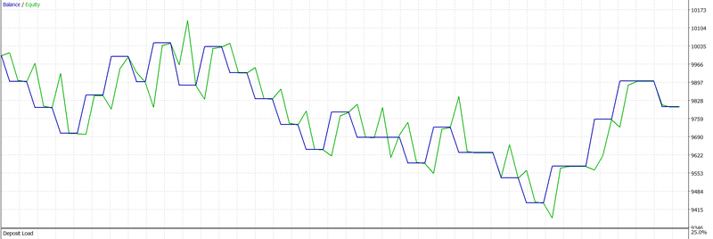
Fig. 2. Balance/equity curve, raw labels (no cleaning). Ends near 9,805 on a 10,000 starting balance.
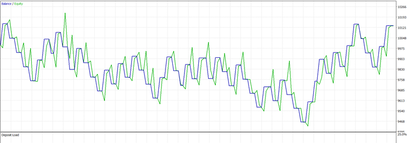
Fig. 3. Balance/equity curve, cleaned labels at pruning aggressiveness 0.25 - the best run of the sweep, ending near 10,134.
Why Aggressive Pruning Backfired
Go back to that guard in CLogRegClassifier::Train: if(n_samples < m_num_features + 2) return(false). With 177 candidates and an estimated 50% prune rate, pruning at full aggressiveness drops the final training set to roughly 88 rows for a 4-feature model. That's not below the hard floor, so training still runs - but it's thin enough that the fitted weights carry a lot of sampling variance from exactly which 88 rows survived the cut, not from any real signal in the remaining data.
Rows available to the final filter at each aggressiveness level, given 177 total candidates:
aggressiveness 1.0 → 177 - 89 = 88 rows trained on
aggressiveness 0.5 → 177 - 45 = 132 rows trained on
aggressiveness 0.25 → 177 - 22 = 155 rows trained on
Put plainly: at full aggressiveness the final model is fit on barely more than half its original training data, for a task where each of the four features is already a fairly weak, noisy signal on its own. A logistic regression with that little data doesn't fail outright - it fits something, and that something can easily be a boundary that happens to separate the surviving 88 rows well without generalizing to the live signals it's asked to approve afterward. That's consistent with what actually happened: the aggressiveness-1.0 filter approved far more trades than either the raw-label model or the more conservatively-cleaned models, which is what you'd expect from a decision boundary shaped more by which rows survived a small cut than by any real structure in the feature space.
There's a second effect stacked on top of that. Pruning at full aggressiveness removes samples per-cell based on the calibrated joint's estimate of the noise count - and that estimate itself comes from a 5-fold cross-fit on only 177 candidates, so each fold's out-of-fold model is trained on roughly 140 rows. A confident joint built from thresholds that shaky is itself noisy, and pruning aggressively on top of a noisy estimate compounds the error rather than correcting it. The auditor isn't wrong to flag 89 rows as suspicious - the calibrated joint math is doing exactly what it's supposed to do given the inputs - but "the auditor's estimate is defensible" and "removing every row it flags is the right policy" turned out to be two different claims.
Backing the aggressiveness down to 0.25 keeps about four-fifths of the flagged rows in the training set - enough to remove the worst, most confidently-mislabeled examples in each cell without starving the classifier of the data it needs to generalize. The sweep is the evidence for that story, not just the reasoning: performance moves monotonically with aggressiveness across all three cleaned runs, in the direction the small-sample argument predicts, and the run with the most training data left over (155 rows, aggressiveness 0.25) is also the run with the best out-of-sample-style trading result.
Testing Beyond EURUSD H1
Everything above is a real result, but it's a result from one symbol on one timeframe, and I don't think that's good enough to call a result on its own - a single symbol/timeframe backtest is closer to an anecdote with a p-value attached. So I went back to the Strategy Tester and ran the same raw-vs-cleaned comparison, at the winning 0.25 aggressiveness setting, on three more symbol/timeframe combinations: EURUSD H4, GBPUSD H1, and USDJPY H1. XAUUSD H1 was the original plan for the fourth combo, but gold wasn't listed on this demo account's Market Watch, and USDJPY satisfies the same "different pair" requirement just as well.
The H4 combo needed one methodology adjustment worth stating plainly rather than burying in a footnote. InpTrainWindowBars, InpRefitEveryBars, and InpLabelHorizonBars are bar counts, not calendar time, so the values tuned for H1 (3000/250/20) represent roughly four times the real-world lookback once you switch to H4. I rescaled them to 750/60/5 to preserve the same ~125-day training window and ~10-day refit cadence, lowered InpMinTrainSamples from 60 to 40 since H4 throws off fewer candidate signals per window than H1 does, and widened the test period to 2025.05.01-2026.09.14 (about 16.5 months) so there was enough runway left after that lookback burned through the front of the window for the EA to actually place a trade. Skip that second adjustment and the test doesn't fail loudly - it just quietly never fires a single trade, which looks like a broken EA but is really just a training window eating the whole backtest.
| Combo | Raw trades | Raw net profit | Raw PF | Raw Sharpe | Cleaned trades | Cleaned net profit | Cleaned PF | Cleaned Sharpe |
|---|---|---|---|---|---|---|---|---|
| EURUSD H1 | 24 | -$194.84 | 0.87 | -1.10 | 57 | +$133.63 | 1.04 | 0.33 |
| EURUSD H4 | 9 | +$94.28 | 1.19 | 0.13 | 22 | -$454.94 | 0.69 | -1.51 |
| GBPUSD H1 | 1 | -$100.32 | 0.00 | -1.66 | 23 | -$770.71 | 0.52 | -4.61 |
| USDJPY H1 | 3 | -$57.16 | 0.71 | -0.09 | 53 | +$128.57 | 1.04 | 0.34 |
Two of the four combos confirm the EURUSD H1 story. USDJPY H1 is close to a carbon copy - a thin, losing raw baseline (three trades, not really enough to trust on its own) turns into a real, moderately profitable filter once trained on cleaned labels, with profit factor and Sharpe landing almost exactly where the EURUSD H1 cleaned run did. The other two flip it entirely. On EURUSD H4, the raw baseline was the one that made money, and cleaning turned a small profit into a real loss. GBPUSD H1's raw baseline only fired once in eight and a half months, so it's barely a baseline at all, but the cleaned version traded 23 times and lost on every metric that matters.
There's a pattern in the two combos where cleaning hurt, and it's a clear one: in both cases the cleaned-label classifier didn't just perform worse, it traded far more often - 22 trades versus 9 on EURUSD H4, 23 versus 1 on GBPUSD H1. That's not a filter getting pickier after removing noisy training rows, it's a filter getting looser. My read, consistent with the small-sample mechanism from the previous section: on a symbol/timeframe combo where the base signal doesn't throw off enough candidates to begin with, pruning shrinks an already-thin training set further, and the resulting decision boundary clears the 0.60 probability threshold more easily without actually getting more accurate.
The honest conclusion here is a mixed one, and I'm not going to sand off the edges to make it a cleaner headline - but I also can't call either direction settled. Two combos moved the way the aggressiveness-sweep story predicts, two moved the opposite way, and every one of those four raw baselines is built on 1 to 24 trades - too few, on their own, to tell a real structural difference between symbols apart from ordinary run-to-run variance. What I can say with more confidence is the mechanism from the previous section: a symbol/timeframe combo that doesn't throw off many candidate signals to begin with is the one where aggressive pruning is most likely to leave the final model short on data, whichever direction that happens to push the result. If you're running this style of audit-and-clean pipeline on your own strategy, validate the pruning step with enough trades on the specific symbol and timeframe you intend to trade, rather than assuming a result that held on one pair transfers automatically to the next.
Limitations and What I'd Test Next
The four-level aggressiveness sweep itself is still one symbol, one timeframe, one eight-and-a-half-month window, and 177 candidate signals total - not enough to call any of these numbers a stable edge, and not enough to claim the 0.25 aggressiveness value is anywhere close to universally optimal even on EURUSD H1. All four numbers in that results table came from the same continuous in-sample window with Forward testing disabled, which means none of them are genuinely out-of-sample in the way a proper walk-forward test would be - the sweep tells you how sensitive this particular pipeline is to one input on one dataset, not how it would perform on data it's never touched in any form.
A few concrete things I'd want before trusting this further. First, a walk-forward split: refit and audit on one window, trade forward on the next, roll the window ahead, and repeat - which is a meaningfully different test than refitting every 250 bars inside one continuous backtest. Second, the full four-level aggressiveness sweep - not just the raw-vs-0.25 comparison in the section above - repeated on the three combos that already have a raw/cleaned data point, to see whether the same monotonic aggressiveness-sensitivity pattern found on EURUSD H1 holds on the combos where cleaning hurt, or whether a softer aggressiveness setting rescues EURUSD H4 and GBPUSD H1 the way it rescued EURUSD H1's full-aggressiveness run. Third, a finer grid around 0.25 rather than the three points tested on EURUSD H1 (1.0, 0.5, 0.25); I only have enough resolution from that sweep to say the optimum sits somewhere between 0.25 and 0.5 on that one combo, not exactly where. Fourth, I'd want to see whether a slightly larger or more heavily-regularized base learner changes how expensive the small-sample effect actually is on the combos where cleaning hurt - a lot of what happened there comes down to fitting a 4-feature model on very few rows, and a model with stronger regularization might tolerate an aggressively-pruned training set better than plain L2 logistic regression did.
I'd also flag the label heuristic itself as a candidate for revision rather than treating it as fixed. InpMinNetMovePoints and InpLabelHorizonBars were both left at their defaults across every run in this sweep - a stricter or more path-aware label (one that actually checks for an intrabar stop-out before scoring a win) might lower the true noise rate on its own, which would be a more fundamental fix than auditing around a label that's noisy by construction.
The other defaults left untouched across every run deserve a sentence each rather than a silent pass. InpProbThreshold=0.60 sits above the no-skill 0.50 line without being so strict that the filter rejects almost everything - it wasn't swept, so treat it as a reasonable starting point, not a tuned optimum. InpTrainWindowBars=3000 (roughly 125 trading days on H1) was picked to span more than one volatility regime without reaching back far enough to train on market structure that's stopped being representative. InpRefitEveryBars=250 (about ten trading days) trades off tracking regime drift against refitting on noise from the last few days alone. None of these three were sensitivity-tested here, and I'm not going to imply they were by leaving them unmentioned - this article is an engineering demonstration of the audit-and-clean mechanism, not a tuned trading strategy, and a real sensitivity sweep on these three belongs in a separate piece with the trade-count budget to support it.
Conclusion
Confident learning did what it's supposed to do here - it found a real, large share of candidates flagged for pruning in a labeling heuristic that has an obvious, documented reason to be noisy, and it did it without a single external ML library, using nothing but a small logistic regression and the cross-fitting/calibration math from Northcutt, Athalye, and Mueller's paper implemented directly in MQL5. What it didn't do, at least not automatically, is improve results just by existing. Pruning every sample the auditor flagged made the live filter worse than doing nothing at all; pruning a quarter as aggressively made it the best run in the sweep.
That gap between "the audit is correct" and "acting on the audit helps" is the actual finding here, and it's the reason I built this as a four-run sensitivity sweep instead of a single before/after comparison. A single comparison at one aggressiveness setting would have shown confident learning failing outright, and I'd have either buried that result or quietly picked a friendlier setting without explaining why. The sweep makes the mechanism visible instead: the auditor's estimate of what's wrong was more reliable than a naive "remove everything it flags" policy for using that estimate, and the reason traces directly back to a training-set-size problem, not a flaw in the audit math itself.
If you build something like this into your own pipeline, treat the pruning-aggressiveness dial as something to sweep and validate on your own data, not something to leave at its most aggressive setting on the assumption that more cleaning is always better. On a small candidate set, the line between "removing noise" and "removing your training data" is closer than it looks.
Programs used in the article
| # | Name | Type | Description |
|---|---|---|---|
| 1 | ConfidentLearningLib.mqh | Include file | Complete MQL5 library implementing the Confident Learning framework. Contains the logistic regression classifier (CLogRegClassifier), label auditor (CConfidentLabelAuditor), and supporting data structures. Provides cross-validation, out-of-fold probability estimation, label quality assessment, noise detection, and removal of potentially mislabeled training samples. Place the file in MQL5/Include/ConfidentLearning/. |
| 2 | ConfidentLearning_Audit_EA.mq5 | Expert Advisor | Complete trading Expert Advisor demonstrating how Confident Learning can improve a meta-labeling strategy. Generates trading signals using RSI and SMA, constructs training labels from subsequent price movements, identifies potentially incorrect labels, and trains a logistic regression trade filter. Supports A/B testing with original and cleaned labels through the InpUseCleanedLabels parameter. Includes periodic model retraining, ATR-based risk management, trade execution, and CSV audit reporting. Place the filein MQL5/Experts/ConfidentLearning/. |
| 3 | ConfidentLearning_FlagView.mq5 | Custom Indicator | Visualization indicator for examining the results of the label audit. Reads the audit_detail.csv file generated by the Expert Advisor and displays self-confidence scores for audited trading signals in a separate indicator window. Marks samples flagged for removal, helping identify potentially unreliable training labels. Run the Expert Advisor first to generate the audit data, then attach the indicator to the corresponding chart. Place the filein MQL5/Indicators/ConfidentLearning/. |
All three source files are included in the archive. The Expert Advisor depends on ConfidentLearningLib.mqh, while the indicator uses the audit report generated by the Expert Advisor.
Warning: All rights to these materials are reserved by MetaQuotes Ltd. Copying or reprinting of these materials in whole or in part is prohibited.
This article was written by a user of the site and reflects their personal views. MetaQuotes Ltd is not responsible for the accuracy of the information presented, nor for any consequences resulting from the use of the solutions, strategies or recommendations described.

 Practical Modules from Other Languages in MQL5 (Part 09): MATPLOTLIB (II)
 How to Replace a WebSocket EA with TradeMux REST in MetaTrader 5
 Features of Experts Advisors
 Crypto Exchange Integration with MQL5 (Part 1): Connecting to MEXC Futures

- Free trading apps
- Over 8,000 signals for copying
- Economic news for exploring financial markets
You agree to website policy and terms of use