Detecting Structural Breakpoints in Price Series Using CUSUM in MQL5 (Part 1): From Statistical Theory to a Working MQL5 Indicator

Introduction

Trading systems often degrade when market regimes shift. Fixed-window indicators such as moving averages or ATR react only after a structural change has already affected prices, because they summarize the recent past rather than test for an active change.

This article presents a sequential alternative based on the Cumulative Sum (CUSUM) control chart. The method processes returns bar by bar, accumulates evidence of a distributional shift, and declares a breakpoint as soon as a statistical threshold is crossed.

The first half explains the statistical construction of the detector: return standardization, dual accumulators, threshold selection, and reset logic. The second half translates the method into a MetaTrader 5 indicator, CUSUM_Breakpoint.mq5, with attention to buffer persistence, recalculation handling, and chart-object management. A second article follows with a full empirical validation across six instruments, three timeframes, and two macroeconomic periods.

The Core Idea

CUSUM watches two running totals built from standardized returns. The moment either one crosses a threshold, a break is declared:

τ=inf{t≥1:S_t^+>h or S_t^-<-h}

Everything in this article explains how S_t^+, S_t^-, and h are built, and exactly what statistical guarantee this single rule provides.

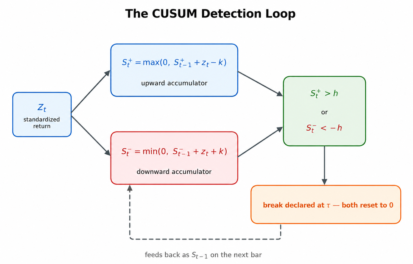
The CUSUM detection loop: a standardized return z_t updates both accumulators every bar; the instant either crosses its threshold, a break is declared and both reset to zero.

Why Regime Shifts Require a Sequential Detector

Financial returns are not generated by a single stable process. Regime shifts in mean, variance, or correlation occur frequently. As a result, models calibrated on a fixed historical window eventually operate on a different distribution than the one they were fitted to. This happens routinely due to central bank decisions, geopolitical shocks, and credit market dislocations. A mean-reversion system calibrated on a calm 200-bar range will produce its worst drawdowns exactly when the instrument transitions into a trend, because the system’s statistical assumptions stop holding the moment the regime changes, not when the equity curve eventually reveals it. Consider EURUSD during a quiet session versus the same pair shortly after an unscheduled central bank statement: every parameter estimated from the calm period describes a different population than the one generating prices afterward.

Conventional indicators do not solve this problem because they are smoothers, not detectors. A moving average or ATR will eventually reflect a new regime, but only after the new observations have already entered the lookback window — by the time the indicator moves, it is describing where the market has been, not the moment it changed. What is needed instead is a sequential hypothesis test that evaluates each new bar as it arrives and signals as soon as enough evidence of change has accumulated, rather than after a fixed window has elapsed.

CUSUM: An Industrial Quality-Control Tool Repurposed for Markets

CUSUM, introduced by E. S. Page in 1954 for industrial process control, is well suited to financial monitoring because it is sequential: it updates a small state on each bar and signals the first time accumulated evidence exceeds a threshold, with no batch reprocessing and no look-ahead bias. For standardized returns z_t, the stopping rule is:

τ=inf{t≥1:S_t^+>h or S_t^-<-h}

Equation (1). The CUSUM stopping rule: a break is declared at the first bar where either accumulator crosses its threshold.

That is the entire detection logic. The rest of this article explains how to make the stopping rule computable and statistically meaningful on real price data: standardization, the choice of h, accumulator behavior, and the MQL5 implementation.

From Price to a Testable Signal: The Standardization Pipeline

Prices are unsuitable for direct sequential testing because they are nonstationary in level. The first transformation is therefore the log-return:

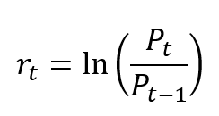
Equation (2). The continuously compounded log-return, converting raw price into a stationary input series.

The second step standardizes the current return using a strictly historical rolling window:

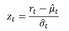
Equation (3). The standardized z-score, using only the strictly historical rolling window ending at t−1.

where μ ̂_t and σ ̂_t are estimated from the previous W returns only, ending at t-1. This produces a dimensionless signal that makes the same threshold h comparable across instruments with different baseline volatility — a z-score of 3 means the same thing on a quiet FX pair or a volatile commodity.

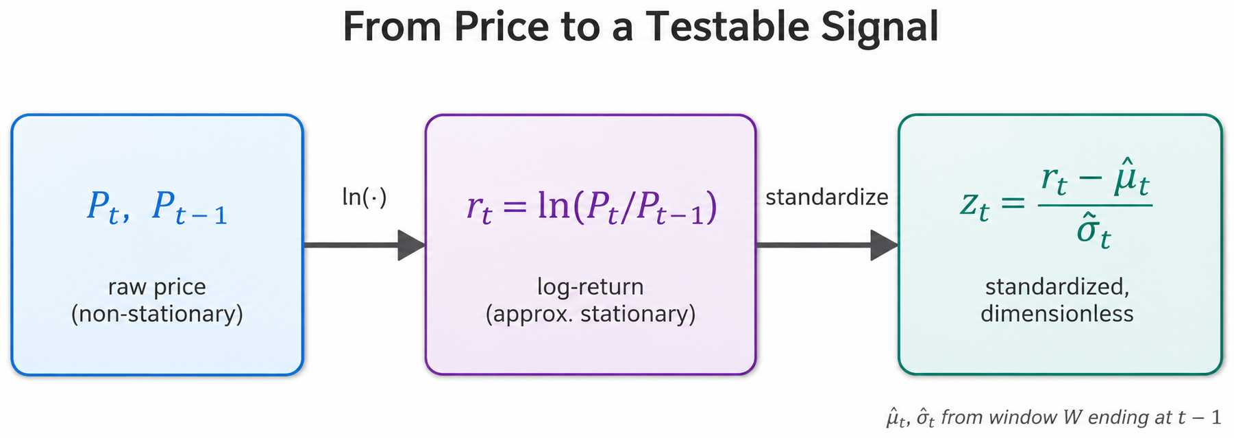
The standardization pipeline: raw price is converted to a log-return, then standardized into a dimensionless z-score using a strictly historical rolling window.

The Dual-Sided Accumulator: Where the Sequential Logic Lives

The CUSUM state is updated by two recurrences:

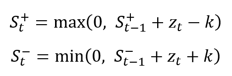
Equations (4) and (5). The dual-sided CUSUM accumulator recurrence: S+ tracks upward drift, S− tracks downward drift.

Their behavior is determined by three properties:

• The clamps keep the two accumulators independent. S^+ never goes negative, S^- never goes positive — each can only push further in its own direction or snap back to zero.
• k acts as an embedded noise allowance. It is subtracted from every positive increment and added to every negative one, so fluctuations smaller than k are absorbed without contributing to the accumulator at all.
• The accumulator reacts to cumulative directional deviation, whether caused by sustained drift or a single extreme bar. Both push the relevant accumulator toward threshold identically — a property the validation results in the second article of this series quantify directly.

In practice, k controls sensitivity. Too small, and ordinary noise accumulates as if it were genuine drift; too large, and real shifts get absorbed into the slack term along with the noise. A common guideline sets k to half the minimum standardized shift worth detecting,

Equation (6). The canonical guideline for the allowance parameter k, set to half the minimum shift worth detecting.

which for most financial applications lands between 0.25 and 0.75.

The Threshold h and the Statistical Guarantee It Provides

The threshold h sets the detector’s core trade-off: smaller values detect faster but increase false alarms, while larger values are more conservative but slower.

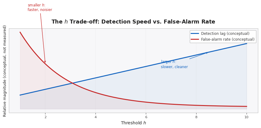
The qualitative shape of the h trade-off: lower thresholds detect faster but tolerate more false alarms; higher thresholds suppress false alarms at the cost of slower confirmation. Shapes are illustrative; Part 2 reports the measured trade-off on real instruments.

This is commonly summarized through the average run length under the null, ARL₀: the expected number of bars between false alarms when no change has occurred. For i.i.d. standard normal inputs, Siegmund’s 1985 approximation provides a closed-form baseline:

Equation (7). Siegmund's 1985 closed-form approximation for the average run length under the null, ARL₀.

Its practical use in finance is limited by the fact that real returns are neither i.i.d. nor exactly normal, so empirical false-alarm rates can differ materially from this theoretical prediction — a gap the second article in this series measures directly, across six instruments, three timeframes, and two distinct macroeconomic periods.

The Reset: What Happens After a Detection

When either accumulator crosses its threshold at time τ, both are immediately reset to zero:

Equation (8). The post-detection reset: both accumulators return to zero immediately after a breakpoint is declared.

This prevents pre-break and post-break evidence from being mixed into the same statistic, and turns each inter-detection interval into a fresh sequential test. This completes the theoretical foundation; the remainder of this article translates Equations (1) through (8) into a working MetaTrader 5 indicator.

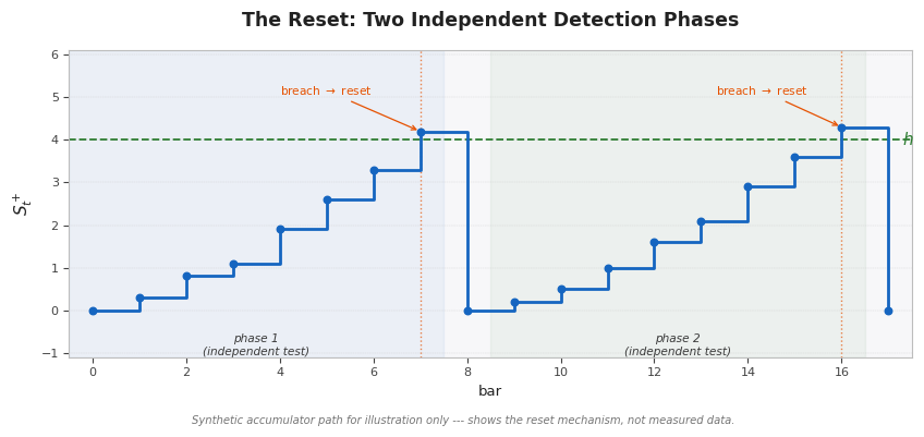
A synthetic illustration of the reset: S_t^+ accumulates, crosses h, and snaps back to zero, beginning a second, fully independent detection phase.

From Mathematics to Software: Three Execution-Model Constraints

Independent implementations often fail during translation to MetaTrader 5 execution. The failures are typically in buffer indexing, state synchronization across recalculation events, and off-by-one errors that may pass a casual backtest but break in live use. A correct implementation must address three execution constraints, and every non-obvious line in the listings below exists to satisfy one of them:

1. Full vs. incremental recalculation: OnCalculate() runs either from scratch (prev_calculated == 0, on initial load, history recalculation, or a timeframe switch) or incrementally on each new tick, where only the newest bars need attention.
2. Persistent state: MQL5 does not reliably preserve ordinary global variables across recalculation events. Accumulator memory — the two scalars S_t^+ and S_t^- — must instead be restored from indicator buffers, which the terminal manages and persists between calls.
3. Idempotent visualization: Each breakpoint must become a chart object exactly once. OnCalculate() is invoked repeatedly while the current bar is still forming, so creating the object without an existence check would flood the terminal with duplicate, failing calls.

The Complete Indicator: Section by Section

Property Block, Plot Declarations, and Inputs

//+------------------------------------------------------------------+
//|                                             CUSUM_Breakpoint.mq5 |
//|           Structural Breakpoint Detector via CUSUM Control Chart |
//+------------------------------------------------------------------+

#property description "Dual-sided CUSUM structural breakpoint detector on log-returns."
#property description "Plots S+ and S- accumulators in a sub-window with ±h boundaries."
#property description "Draws vertical lines on the main chart at every declared breakpoint."

//--- Indicator windows and buffer allocations
#property indicator_separate_window
#property indicator_buffers 6
#property indicator_plots   4

//--- Plot 1: Positive CUSUM Accumulator (S+)
#property indicator_label1  "S+"
#property indicator_type1   DRAW_LINE
#property indicator_color1  clrDodgerBlue
#property indicator_style1  STYLE_SOLID
#property indicator_width1  2

//--- Plot 2: Negative CUSUM Accumulator (S-)
#property indicator_label2  "S-"
#property indicator_type2   DRAW_LINE
#property indicator_color2  clrOrangeRed
#property indicator_style2  STYLE_SOLID
#property indicator_width2  2

//--- Plot 3: Upper Detection Boundary (+h)
#property indicator_label3  "+h Threshold"
#property indicator_type3   DRAW_LINE
#property indicator_color3  clrLimeGreen
#property indicator_style3  STYLE_DOT
#property indicator_width3  1

//--- Plot 4: Lower Detection Boundary (-h)
#property indicator_label4  "-h Threshold"
#property indicator_type4   DRAW_LINE
#property indicator_color4  clrMagenta
#property indicator_style4  STYLE_DOT
#property indicator_width4  1

//--- Input Parameters
input int    inp_CalibrationWindow    = 100;          // Rolling window size for mean and variance calibration
input double inp_AllowanceK           = 0.50;         // Slack/Drift parameter (k) in standard deviations
input double inp_ThresholdH           = 4.00;         // Critical decision threshold (h) for break detection
input int    inp_VLineWidth           = 2;            // Breakpoint vertical line thickness
input color  inp_VLineColor           = clrYellow;    // Breakpoint vertical line color
input int    inp_MinBarsBetweenBreaks = 10;           // Refractory period (minimum gap between structural breaks)

//--- Global Indicator Buffers
double g_BufSplus[];
double g_BufSminus[];
double g_BufUpperH[];
double g_BufLowerH[];
double g_BufLogReturn[];
double g_BufZScore[];

//--- Global State Tracking Variables
int    g_LastBreakBar    = -1;                     // Index of the most recently flagged structural break
int    g_TotalBarsOnInit = 0;                      // Cached historical bar count at initialization
string g_IndicatorName   = "CUSUM_BP";             // Prefix string used for chart object management

Six buffers are declared because four are plotted and two store intermediate calculations (log returns and z-scores). The latter are registered as INDICATOR_CALCULATIONS so they persist across calls without being rendered. g_LastBreakBar lives outside the buffer system since its only job is suppressing rapid repeated detections, not holding mathematical state.

Input Parameter Reference

Before stepping through the rest of the logic, here is what every input does and how it changes the indicator’s behavior. Read this as the configuration map you will return to when tuning the indicator on different instruments — and as the starting point for the empirical calibration question the second article in this series answers in full.

Parameter	Default	Valid range	Practical effect
inp_CalibrationWindow	100	≥10	Rolling window W used to estimate μ ̂_t and σ ̂_t. Larger windows give a more stable standardization but react more slowly to a genuine change in baseline volatility.
inp_AllowanceK	0.50	>0	The allowance k from Equation (6). Controls how much standardized deviation is absorbed as noise before it contributes to either accumulator.
inp_ThresholdH	4.00	>0	The detection threshold h. Smaller values detect faster but tolerate more false alarms; see the trade-off discussion above and the measured values in the second article of this series.
inp_VLineWidth	2	≥1	Pixel width of the vertical breakpoint markers drawn on the main chart.
inp_VLineColor	clrYellow	any color	Color of the vertical breakpoint markers.
inp_MinBarsBetweenBreaks	10	≥1	Refractory period: the minimum bar gap enforced between two consecutive declared breaks, preventing rapid repeated detections immediately after a reset.

A practical starting profile for most FX instruments on H1: keep the defaults and adjust h first if the breakpoint frequency looks too high or too low for the instrument in question — k and W are usually the last parameters worth touching.

OnInit(): Validation and Buffer Registration

//+------------------------------------------------------------------+
//| Custom indicator initialization function                         |
//+------------------------------------------------------------------+
int OnInit()
  {
//--- Validate input boundaries to avoid runtime zero-division or logical failures
   if(inp_CalibrationWindow < 10)
     {
      Print("CUSUM ERROR: inp_CalibrationWindow must be >= 10. Received: ",
            inp_CalibrationWindow);
      return(INIT_PARAMETERS_INCORRECT);
     }
   if(inp_AllowanceK <= 0.0)
     {
      Print("CUSUM ERROR: inp_AllowanceK must be strictly positive. Received: ",
            inp_AllowanceK);
      return(INIT_PARAMETERS_INCORRECT);
     }
   if(inp_ThresholdH <= 0.0)
     {
      Print("CUSUM ERROR: inp_ThresholdH must be strictly positive. Received: ",
            inp_ThresholdH);
      return(INIT_PARAMETERS_INCORRECT);
     }
   if(inp_MinBarsBetweenBreaks < 1)
     {
      Print("CUSUM ERROR: inp_MinBarsBetweenBreaks must be >= 1. Received: ",
            inp_MinBarsBetweenBreaks);
      return(INIT_PARAMETERS_INCORRECT);
     }

//--- Map indicator arrays to explicit structural data and calculation channels
   SetIndexBuffer(0, g_BufSplus,      INDICATOR_DATA);
   SetIndexBuffer(1, g_BufSminus,     INDICATOR_DATA);
   SetIndexBuffer(2, g_BufUpperH,     INDICATOR_DATA);
   SetIndexBuffer(3, g_BufLowerH,     INDICATOR_DATA);
   SetIndexBuffer(4, g_BufLogReturn,  INDICATOR_CALCULATIONS);
   SetIndexBuffer(5, g_BufZScore,     INDICATOR_CALCULATIONS);

//--- Define values to be ignored by the visual rendering engine
   PlotIndexSetDouble(0, PLOT_EMPTY_VALUE, EMPTY_VALUE);
   PlotIndexSetDouble(1, PLOT_EMPTY_VALUE, EMPTY_VALUE);
   PlotIndexSetDouble(2, PLOT_EMPTY_VALUE, EMPTY_VALUE);
   PlotIndexSetDouble(3, PLOT_EMPTY_VALUE, EMPTY_VALUE);

//--- Configure the sub-window shorthand dynamic label string
   IndicatorSetString(INDICATOR_SHORTNAME,
                      StringFormat("CUSUM(W=%d, k=%.2f, h=%.2f)",
                                   inp_CalibrationWindow,
                                   inp_AllowanceK,
                                   inp_ThresholdH));

//--- Configure static horizontal sub-window reference levels
   IndicatorSetDouble(INDICATOR_LEVELVALUE,   0, inp_ThresholdH);
   IndicatorSetDouble(INDICATOR_LEVELVALUE,   1, -inp_ThresholdH);
   IndicatorSetInteger(INDICATOR_LEVELCOLOR,  0, clrLimeGreen);
   IndicatorSetInteger(INDICATOR_LEVELCOLOR,  1, clrMagenta);
   IndicatorSetInteger(INDICATOR_LEVELSTYLE,  0, STYLE_DOT);
   IndicatorSetInteger(INDICATOR_LEVELSTYLE,  1, STYLE_DOT);

//--- Offset plot rendering to ensure the calibration window has completely warmed up
   PlotIndexSetInteger(0, PLOT_DRAW_BEGIN, inp_CalibrationWindow + 1);
   PlotIndexSetInteger(1, PLOT_DRAW_BEGIN, inp_CalibrationWindow + 1);
   PlotIndexSetInteger(2, PLOT_DRAW_BEGIN, inp_CalibrationWindow + 1);
   PlotIndexSetInteger(3, PLOT_DRAW_BEGIN, inp_CalibrationWindow + 1);

//--- Flush historical operational variables
   g_LastBreakBar    = -1;
   g_TotalBarsOnInit = iBars(_Symbol, _Period);

   return(INIT_SUCCEEDED);
  }

OnInit() validates inputs, registers the data and calculation buffers, sets the threshold reference levels, and delays plotting until the calibration window is fully warmed up — the +1 in PLOT_DRAW_BEGIN accounts for the single bar of lag the log-return transformation introduces at the start of any series.

OnDeinit(): Cleaning Up Chart Objects

//+------------------------------------------------------------------+
//| Custom indicator deinitialization function                       |
//+------------------------------------------------------------------+
void OnDeinit(const int reason)
  {
//--- Isolate and wipe indicator-generated vertical lines from the current chart space
   string vline_prefix  = g_IndicatorName + "_VL_";
   int    total_objects = ObjectsTotal(0, 0, OBJ_VLINE);

   for(int i = total_objects - 1; i >= 0; i--)
     {
      string obj_name = ObjectName(0, i, 0, OBJ_VLINE);
      if(StringFind(obj_name, vline_prefix) == 0)
         ObjectDelete(0, obj_name);
     }

//--- Clear state identifiers
   g_LastBreakBar    = -1;
   g_TotalBarsOnInit = 0;

   Print("CUSUM_Breakpoint: All chart objects removed. Deinitialization complete. Reason: ",
         reason);
  }

OnDeinit() removes only the vertical lines created by this indicator instance, identified by a shared name prefix, walking the object list backward so each deletion does not shift the indices of objects not yet visited.

OnCalculate(): The Three-Pass Engine

The calculation engine runs as sequential passes, each depending on the output of the one before it: standardization needs the full log-return series before computing a rolling mean and standard deviation, and the CUSUM recurrence needs the standardized z-score before it can update either accumulator.

//+------------------------------------------------------------------+
//| Custom indicator iteration function                              |
//+------------------------------------------------------------------+
int OnCalculate(const int rates_total,
                const int prev_calculated,
                const datetime &time[],
                const double   &open[],
                const double   &high[],
                const double   &low[],
                const double   &close[],
                const long     &tick_volume[],
                const long     &volume[],
                const int      &spread[])
  {
//--- Enforce minimum data requirements before executing calculations
   if(rates_total < inp_CalibrationWindow + 2)
      return(0);

//--- Determine historical data processing entry bar
   int start_bar;
   if(prev_calculated == 0)
     {
      //--- Wipe previous indicator objects if full recalculation is triggered
      string vline_prefix  = g_IndicatorName + "_VL_";
      int    total_objects = ObjectsTotal(0, 0, OBJ_VLINE);
      for(int i = total_objects - 1; i >= 0; i--)
        {
         string obj_name = ObjectName(0, i, 0, OBJ_VLINE);
         if(StringFind(obj_name, vline_prefix) == 0)
            ObjectDelete(0, obj_name);
        }
      g_LastBreakBar = -1;
      start_bar      = 1; // Begin at the first valid relative close shift
     }
   else
     {
      //--- Re-evaluate the last calculated bar to account for tick fluctuations on live candles
      start_bar = prev_calculated - 1;
      if(start_bar < 1)
         start_bar = 1;
     }

prev_calculated separates full-history initialization from incremental updates. On live ticks, the last processed bar is recalculated because its close may still be changing, and any stale chart objects from a full recalculation are cleared before new ones are created.

//--- Step 1: Calculate continuous logarithmic close-to-close returns
   for(int bar = start_bar; bar < rates_total; bar++)
     {
      if(close[bar] <= 0.0 || close[bar - 1] <= 0.0)
        {
         g_BufLogReturn[bar] = 0.0;
         continue;
        }
      g_BufLogReturn[bar] = MathLog(close[bar] / close[bar - 1]);
     }
   g_BufLogReturn[0] = 0.0; // Terminal anchor point

This pass implements Equation 2 directly. The guard against non-positive close prices avoids feeding MathLog() an undefined input on synthetic or back-adjusted instruments during contract rolls.

//--- Step 2: Calculate rolling historical Z-Scores via statistical vectors
   int zscore_start = (prev_calculated == 0) ? inp_CalibrationWindow : start_bar;
   if(zscore_start < inp_CalibrationWindow)
      zscore_start = inp_CalibrationWindow;

   for(int bar = zscore_start; bar < rates_total; bar++)
     {
      vector v_window;
      v_window.Init(inp_CalibrationWindow);

      //--- Extract historical returns for the current execution frame
      for(int w = 0; w < inp_CalibrationWindow; w++)
        {
         int window_idx = bar - 1 - w;
         if(window_idx < 0)
            v_window[w] = 0.0;
         else
            v_window[w] = g_BufLogReturn[window_idx];
        }

      double rolling_mean    = v_window.Mean();
      double rolling_std_pop = v_window.Std(); // Outputs population standard deviation
      double n_dbl           = (double)inp_CalibrationWindow;
      double rolling_std;

      //--- Guard against division-by-zero errors in non-volatile or flat series
      if(rolling_std_pop < 1e-10)
        {
         g_BufZScore[bar] = 0.0;
         continue;
        }
      else
        {
         //--- Convert population standard deviation to unbiased sample standard deviation (Bessel's correction)
         rolling_std = rolling_std_pop * MathSqrt(n_dbl / (n_dbl - 1.0));
        }

      //--- Map standardized returns to the processing calculation buffer
      g_BufZScore[bar] = (g_BufLogReturn[bar] - rolling_mean) / rolling_std;
     }

The z-score uses only the previous W returns, excluding the current bar to avoid look-ahead bias, with Bessel’s correction applied to convert the population standard deviation to the sample estimate. A near-zero standard deviation is guarded against to prevent division by zero on flat or illiquid segments.

//--- Step 3: Zero-out or warm up initial indexes beneath the calibration threshold
   for(int bar = 0; bar < inp_CalibrationWindow && bar < rates_total; bar++)
     {
      g_BufZScore[bar]  = EMPTY_VALUE;
      g_BufSplus[bar]   = EMPTY_VALUE;
      g_BufSminus[bar]  = EMPTY_VALUE;
      g_BufUpperH[bar]  = EMPTY_VALUE;
      g_BufLowerH[bar]  = EMPTY_VALUE;
     }

Every bar inside the calibration window has no valid z-score, so this pass marks the five relevant buffers as EMPTY_VALUE across that range, which the terminal’s rendering engine skips rather than connecting into the plotted line.

//--- Step 4: Core cumulative sum (CUSUM) state tracking preparation
   double S_plus, S_minus;
   int    cusum_start;

   if(prev_calculated == 0)
     {
      cusum_start = inp_CalibrationWindow;
      S_plus      = 0.0;
      S_minus     = 0.0;
     }
   else
     {
      //--- Restore accumulator states from the bar prior to the current parsing step
      cusum_start   = start_bar;
      int prior_bar = cusum_start - 1;

      if(prior_bar < inp_CalibrationWindow ||
         g_BufSplus[prior_bar]  == EMPTY_VALUE ||
         g_BufSminus[prior_bar] == EMPTY_VALUE)
        {
         S_plus  = 0.0;
         S_minus = 0.0;
        }
      else
        {
         S_plus  = g_BufSplus[prior_bar];
         S_minus = g_BufSminus[prior_bar];
        }
     }

On incremental calls, the accumulator state is restored from the previous bar’s buffers, which serve as the indicator’s persistent memory — this is the entire mechanism by which S_t^+ and S_t^- survive from one tick to the next.

//--- Step 5: Execute dual-sided CUSUM recurrence and structural breach validation
   for(int bar = MathMax(cusum_start, inp_CalibrationWindow); bar < rates_total; bar++)
     {
      if(g_BufZScore[bar] == EMPTY_VALUE)
        {
         g_BufSplus[bar]  = EMPTY_VALUE;
         g_BufSminus[bar] = EMPTY_VALUE;
         g_BufUpperH[bar] = EMPTY_VALUE;
         g_BufLowerH[bar] = EMPTY_VALUE;
         continue;
        }

      double zt = g_BufZScore[bar];

      //--- Non-linear recurrence equations mapping cumulative variance deviations
      S_plus  = MathMax(0.0, S_plus  + zt - inp_AllowanceK);
      S_minus = MathMin(0.0, S_minus + zt + inp_AllowanceK);

      //--- Commit calculation states to viewable indicators
      g_BufSplus[bar]  = S_plus;
      g_BufSminus[bar] = S_minus;
      g_BufUpperH[bar] = inp_ThresholdH;
      g_BufLowerH[bar] = -inp_ThresholdH;

      //--- Assess if statistical boundary breaches occurred on the current bar
      bool upper_breach = (S_plus  >  inp_ThresholdH);
      bool lower_breach = (S_minus < -inp_ThresholdH);

      if(upper_breach || lower_breach)
        {
         //--- Verify structural time constraints (refractory minimum gap window)
         bool gap_ok = (g_LastBreakBar < 0) ||
                       ((bar - g_LastBreakBar) >= inp_MinBarsBetweenBreaks);
         if(gap_ok)
           {
            g_LastBreakBar = bar;
            string vline_name = g_IndicatorName + "_VL_" + IntegerToString(bar);

            //--- Instantiate visualization markers for the structural breakpoint
            if(ObjectFind(0, vline_name) < 0)
              {
               ObjectCreate(0, vline_name, OBJ_VLINE, 0, time[bar], 0);
               ObjectSetInteger(0, vline_name, OBJPROP_COLOR,      inp_VLineColor);
               ObjectSetInteger(0, vline_name, OBJPROP_STYLE,      STYLE_DASH);
               ObjectSetInteger(0, vline_name, OBJPROP_WIDTH,      inp_VLineWidth);
               ObjectSetInteger(0, vline_name, OBJPROP_SELECTABLE, false);
               ObjectSetInteger(0, vline_name, OBJPROP_HIDDEN,     true);
               ObjectSetString(0,  vline_name, OBJPROP_TOOLTIP,
                               StringFormat("CUSUM Break | Bar %d | %s",
                                            bar,
                                            TimeToString(time[bar],
                                                  TIME_DATE | TIME_MINUTES)));
              }
           }
         //--- Reset accumulators immediately upon breach verification to start tracking new regime shifts
         S_plus  = 0.0;
         S_minus = 0.0;
        }
     }

   return(rates_total);
  }

MathMax(0.0, S_plus + zt - inp_AllowanceK) and MathMin(0.0, S_minus + zt + inp_AllowanceK) are a direct, line-for-line translation of Equations (4) and (5). Before creating a vertical line, the code checks whether the object already exists — this keeps marker creation idempotent during repeated OnCalculate() calls on the same live bar. The reset to zero immediately after a breach is the software implementation of Equation (8).

Installing and Viewing the Indicator

1. Open MetaEditor (F4 in MetaTrader 5).
2. Go to File → New → Custom Indicator.
3. Name it CUSUM_Breakpoint, paste the complete source from the section above, and press Compile (F7). Confirm the compiler reports zero errors and zero warnings.
4. In MetaTrader 5, open any chart, go to Insert → Indicators → Custom, and select CUSUM_Breakpoint.
5. Set your parameters in the input dialog — the defaults from the Input Parameter Reference Table above are a reasonable starting point — and click OK.

The indicator opens in its own sub-window, plotting S_t^+ in blue and S_t^- in orange-red against two dotted reference lines at +h and -h. On the main chart, a vertical line appears at every bar where a breakpoint was declared — this is the reproducible output the rest of this article has been building toward.

CUSUM_Breakpoint attached to a EURUSD H1 chart. The S+ accumulator (blue, sub-window) crosses the +4.0 threshold at 2026.06.15 00:00, triggering a declared breakpoint — marked by the yellow vertical line on the main chart — immediately followed by a reset to zero. The breakpoint coincides with the start of the visible upward move in price.

Practical Usage Patterns

Reading Breakpoints from an Expert Advisor

The indicator’s accumulator buffers are readable from any EA or script via iCustom() and CopyBuffer(). A minimal single-symbol check looks like this:

int handle = iCustom(_Symbol, _Period, "CUSUM_Breakpoint",
                     100, 0.50, 4.00, 2, clrYellow, 10);

double s_plus[1], s_minus[1];

if(CopyBuffer(handle, 0, 1, 1, s_plus) > 0 &&
   CopyBuffer(handle, 1, 1, 1, s_minus) > 0)
  {
   if(s_plus[0] > 4.00 || s_minus[0] < -4.00)
     {
      //--- A breakpoint was declared on the most recently closed bar
      Print("CUSUM breakpoint detected at bar 1");
     }
  }

As a Volatility-Regime Gate

Given what the dual-accumulator construction section establishes about what this detector responds to, the indicator is best used as a gate rather than a directional signal: pause a mean-reversion system, widen stop distances, or reduce position size for a fixed number of bars immediately after a breakpoint, rather than treating the breakpoint itself as a buy or sell trigger. The breakpoint says the recent return distribution has shifted; it does not say which direction price will move next.

Combining With a Trend or Mean-Reversion Filter

A common pattern is to run the CUSUM detector alongside an existing system purely as a risk overlay: the underlying system continues generating its own entries and exits, and the CUSUM breakpoint state is checked only to decide whether the system’s normal position sizing should apply, or be reduced, on the current bar. This keeps the statistical detector decoupled from the entry logic entirely, which avoids quietly conflating "a structural break happened" with "trade in this direction."

Understanding the Implementation’s Limitations

The limitations below are properties of this specific code, distinct from the statistical limitations of the CUSUM method itself, which the second article in this series quantifies in full across six instruments. These are implementation constraints worth knowing before you deploy or modify the indicator.

• No intrabar accumulator update: The accumulators advance once per closed bar; a breakpoint is confirmed only after the triggering bar closes, so detection latency always includes at least the remainder of the bar in progress.
• Strictly positive prices are assumed: Instruments that can present a zero or negative price during a contract roll will have those bars silently treated as a zero return.
• History depth affects the exact accumulator path: A chart loaded with two years of history and the same chart loaded with five years can diverge slightly within the first calibration window after load, though this disappears beyond it.
• A terminal reconnect forces a full recalculation: A momentary disconnection can produce a brief visual flicker as objects are cleared and redrawn; this is expected behavior, not a malfunction.

Conclusion

This article established the theoretical framework for a CUSUM-based breakpoint detector and detailed its translation into a functional MetaTrader 5 indicator. Replacing conventional fixed-window smoothing with a sequential statistical test on standardized log-returns, the methodology utilizes dual accumulators governed by an allowance parameter (k), a decision threshold (h), and a post-detection reset mechanism. The underlying MQL5 software architecture preserves internal accumulator states across execution cycles using terminal indicator buffers, manages logical branching between full historical recalculations and real-time updates, and renders deterministic breakpoint markers directly onto the chart.

Theoretical guarantees for h and ARL₀ assume i.i.d. normal returns. Empirical financial data routinely violates these assumptions, so practical validity requires rigorous historical testing. The second article in this series addresses this limitation by executing an empirical validation battery across six instruments, three timeframes, and two distinct macroeconomic regimes. This forthcoming study compares real-world false-positive rates with Siegmund's theoretical prediction. It also tests whether detected breakpoints correspond to shifts in mean or variance, and quantifies how much the textbook formula underestimates empirical false-signal frequency.

Program used in the article:

#	Name	Type	Description
1	CUSUM_Breakpoint.mq5	Custom Indicator	A dual-sided CUSUM structural breakpoint detector operating on standardized log-returns. It plots both accumulators against ±h threshold boundaries in a dedicated sub-window and marks every declared breakpoint as a vertical line on the main chart.