

Creating a Cairo-Inspired Graphics Library for MetaTrader 5 (Part 6): Curves and Adaptive Flattening
 669
 0

Contents
- Introduction
- What a Bézier curve is
- Store the curves, or flatten them?
- The flatness test
- De Casteljau: splitting with nothing but midpoints
- Why adaptive beats a fixed segment count
- The tolerance, and the setting it is not
- The two curve verbs
- The demo
- Project structure
- What this does not solve, and what is in Part 7
Introduction
A vector graphics library that can only draw straight lines has a fundamental limitation: no matter how capable its rasterizer is, every curved shape must first be approximated by a polygon. A circle becomes a collection of short segments, and its apparent smoothness depends entirely on how many segments were chosen.
By the end of Part 5, our engine could fill any outline it was given. Edges were smooth at any angle, alpha compositing was correct, and two fill rules allowed shapes to contain holes. That is a capable renderer, but it still cannot draw a curve.
Every "circle" in the last three demos was a polygon whose vertices the demo computed by hand. That made a useful point at the time — the rasterizer cannot tell a 96-sided polygon from a circle, and does not want to — but it is not a library feature. You cannot ask this library for a curve. You can only ask it for a great many short straight lines and hope you asked for the right number of them.
In this part, we add the real thing: CurveTo, the cubic Bézier. The curve itself is four points and some averaging, and on its own it would be a short article. What makes it a long one is the question every vector renderer has to answer, and which has no obvious right answer:
A curve is smooth and infinitely detailed. Our rasterizer eats straight segments. How many segments, and where?
Too few and a circle looks like a stop sign. Too many and you spend time on detail that does not survive being drawn. Pick a number in the middle and you are wrong in both directions at once, because the same number has to serve a four-pixel corner radius and a four-hundred-pixel arc in the same window.
The answer is one of the most satisfying algorithms in computer graphics. It is about thirty lines long and decades old: Paul de Casteljau developed the underlying subdivision method while working at Citroën in 1959, and its central idea remains just as useful today.
Here is the state of the library as this part begins, and what it gains.
Color.mqh      Part 1    the ARGB color type
               Part 4    + CairoBlendOver
Config.mqh     Part 4    CairoAaSamples - the AA quality dial
               Part 6    + CairoFlattenTolerance                     <- today
Surface.mqh    Part 1    a pixel buffer bound to one chart object
Path.mqh       Part 2    points, contours, the pen
               Part 3    + BuildEdges
               Part 5    + AddThickLine
               Part 6    + CurveTo, QuadTo, the flattener            <- today
Raster.mqh     Part 3/4  the scanline fill, with coverage
               Part 5    + the fill rule
Notice what is not in that list. Raster.mqh is untouched today — not "barely changed", not "one small case added". Not one line. That was the promise the architecture made in Part 1, and this is the article where it pays.
What a Bézier curve is
A cubic Bézier is defined by four points:
- P0 — where the curve starts;
- P1, P2 — two control points;
- P3 — where the curve ends.
The curve passes through P0 and P3. In the general case it does not pass through P1 and P2 — it is pulled towards them and does not normally reach them. That sounds like an odd way to define a shape until you have dragged a handle in a design tool for five minutes, at which point it becomes the only way that feels natural.
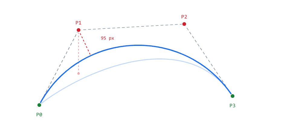
Figure 1. A cubic Bézier: the curve reaches the green points, not the red.
Figure 1 makes the "pulled towards" part concrete. The dashed grey lines are the control polygon — P0 to P1, P1 to P2, P2 to P3 — which is what those little handles in a design tool are drawing. The pale curve behind the blue one is the same call with P1 dragged downwards: the whole shape follows the point without ever reaching it. The dashed red line measures the closest the blue curve ever comes to P1, and the answer is 95 pixels. It does not close.
Two properties matter for everything that follows, and both are worth carrying in your head rather than looking up.
The tangent at each end points along the control polygon. The curve leaves P0 heading directly at P1, and arrives at P3 heading directly from P2. That is what makes Béziers easy to join smoothly: put the outgoing handle of one curve on the same line as the incoming handle of the next, and the joint is invisible. It is also why those handles are drawn as lines from the point rather than as free-floating dots.
The curve always lies inside the convex hull of its four points. It can never escape the hull those points define — a quadrilateral in the general case, but a triangle, a segment or even a single point when the points coincide or are collinear. This is not a rule of thumb, it is a consequence of the way the curve is defined, and the whole flattening algorithm below is built on it. If you remember one property from this section, remember this one.
Cubic Béziers are the universal currency of vector graphics: SVG's C command, PostScript's curveto, PDF paths all reduce to this curve. OpenType is the one format that needs care, because it can carry outlines in two flavours: CFF outlines, which are cubic, and TrueType outlines (which OpenType also wraps), which are quadratic. Every quadratic is exactly representable as a cubic, so a cubic-capable library can consume both — that is what the QuadTo verb later in this article is for. Adding cubics is what makes the library able to consume geometry that came from somewhere else, rather than only geometry that was typed into it.
Store the curves, or flatten them?
There are several ways to support curves in a renderer, and the choice shapes everything downstream — so it is worth making deliberately rather than by accident. Two of them dominate, and the two intermediate strategies are worth naming even though we do not pick them.
Option 1 — keep curves as curves. Add a segment type to the path, so it holds a mixture of lines and curves, and teach everything downstream to handle both.
This is what a full retained-mode system does, and it has real advantages. The path stays compact: four points instead of forty. And because the curve is still a curve, it can be re-flattened at a different resolution when it is transformed or zoomed, so scaling a path up by ten does not reveal facets.
The cost is that BuildEdges needs a curve case, and so does anything else that ever walks a path. Every future feature has to handle two kinds of segment forever, and "forever" in a library that intends to reach a widget toolkit is a long time.
Intermediate options. A renderer can keep the analytic path but flatten lazily, at the moment the path is first rasterized (or first walked by any consumer) rather than at the moment CurveTo is called. It can cache a flattened representation alongside the analytic one, so repeated draws at one size are cheap and a resize triggers a re-flatten. Or it can store the analytic path and tessellate in device space, which is what a zoomable canvas needs. All three keep the path re-flattenable at the cost of a richer path object and a tessellation step that has to be wired into every consumer. They are the right choice for different programs; they are not what this article picks, and the reason is the next paragraph.
Option 2 — flatten immediately. CurveTo converts the curve into short straight segments at the moment it is called, and appends them to the very same vertex array that MoveTo and LineTo have been filling since Part 2.
We take option 2. Here is the trade, stated honestly in both directions.
What we lose: a path is fixed at the resolution it was built for. Scale a flattened path up by 10x and the facets show. In practice this costs us close to nothing, because UI code rebuilds its paths whenever sizes change anyway — a panel that is resized redraws, and a redraw rebuilds. If you were writing a zoomable vector editor, this would be the wrong choice, and it is worth knowing which kind of program you are writing before you copy the decision.
What we gain:nothing downstream changes, ever. BuildEdges does not learn about curves. The rasterizer does not learn about curves. The fill rules, the coverage arithmetic, the compositing pass — untouched. A path containing a two-thousand-segment flattened curve and a path containing a triangle are the same kind of object, and every function that has ever taken a path keeps working without being told anything. That guarantee holds for the filling path this article is about. It does not extend to operations that would need the original analytic curve — transformations, dashed strokes, hit testing, length measurement, morphing — because once the vertices are flattened, the curve is gone. Those features, when they arrive, will need either a richer path object or a re-flatten at the point of use.
This is the same choice Part 5 made with strokes: build the feature out of what already exists rather than teaching the core a new concept. It is the reason the whole engine is still comfortably under two thousand lines, and the reason each article has been able to add a capability rather than a special case.
The flatness test
So: given four points, when is a curve straight enough to be replaced by a single line?
Go back to the convex hull property. The curve cannot escape the convex hull of its four points. So if both control points lie very close to the chord P0→P3, the curve has almost nowhere to go — the hull it is trapped in is barely thicker than the chord itself, so the curve must lie close to that chord too.
That gives a test which is cheap and conservative. Measure the perpendicular distance from each control point to the chord; if the two distances together are within our tolerance, emit the chord and stop.
Here is the measurement, and it is the first of the four functions this part adds to Path.mqh:
double CCairoPath::DistanceToChord( const double px, const double py,
                                    const double ax, const double ay,
                                    const double bx, const double by )
{
    const double dx   = bx - ax;
    const double dy   = by - ay;
    const double len2 = dx * dx + dy * dy;

    //--- degenerate chord (a == b): no line to measure against, so
    //--- fall back to plain point-to-point distance. The test is on
    //--- the SQUARED length, which keeps the square root out of the
    //--- branch that is about to return early anyway.
    if( len2 < 1e-12 )
    {
        const double ex = px - ax;
        const double ey = py - ay;

        return MathSqrt( ex * ex + ey * ey );
    }

    const double cross = ( px - ax ) * dy - ( py - ay ) * dx;

    return MathAbs( cross ) / MathSqrt( len2 );
}
The mathematics is the 2D cross product, and it is worth seeing why it works rather than trusting it. The magnitude of the cross product of two vectors is the area of the parallelogram they span. Take the two vectors a→b and a→p: the parallelogram they span has base |a→b|, and its height is the perpendicular distance from p to the line through a and b. Area divided by base is height.
That is the whole derivation, and it is why the function contains no trigonometry, no special case for a vertical chord, and exactly one call to MathSqrt. Try writing the same measurement from the line equation y = mx + c and you will need a separate branch the moment the chord becomes vertical and m becomes infinite. The cross product has no such direction to be afraid of.
Work one number through it. Take the chord from a = (0, 0) to b = (100, 0) and the control point p = (30, 4). Then dx = 100, dy = 0, len2 = 10000, and cross = 30 * 0 - 4 * 100 = -400. The absolute value is 400, the square root of len2 is 100, and the answer is 4 — which is obviously right for a horizontal chord, and is arrived at by code that never noticed the chord was horizontal.
The len2 computed but not square-rooted until the last line is deliberate. The degenerate test compares a squared length against a squared threshold, which keeps MathSqrt out of the branch that is about to return early. It is a small saving in a function that runs several times per segment of every curve in the interface.
The degenerate branch itself handles a curve whose two endpoints coincide — a loop, where the "chord" is a single point and there is no line to measure against. That is not a hypothetical case invented to look thorough: a closed shape built by a loop over an angle produces exactly this situation every time the loop wraps, and without the branch the division would be by zero.
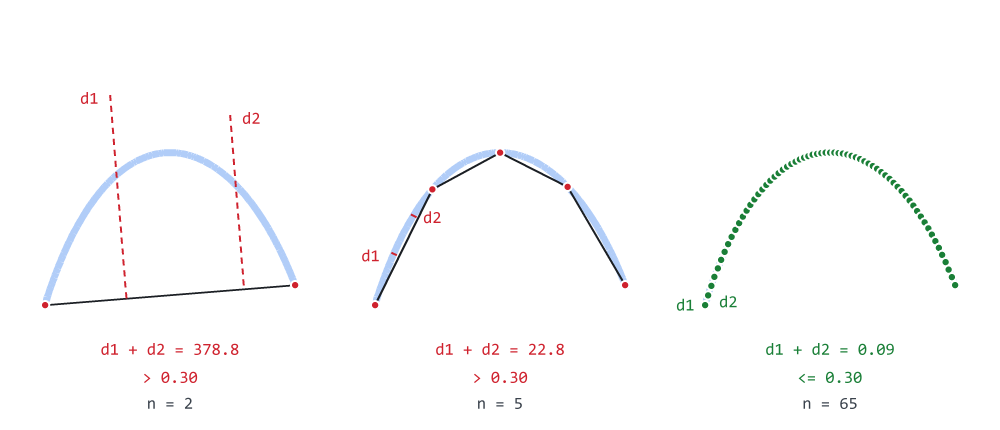
Figure 2. One curve, split until every piece passes the flatness test.
Figure 2 is the test driving the recursion, measured rather than drawn by eye. The pale blue shape is the true curve in all three panels; the black lines are the chords that would actually be emitted; the dots are the vertices. In the first panel there is one chord, and the largest d1 + d2 among the pieces is 378.8 — nowhere near the 0.30 default, so it splits. After two levels there are four chords and the worst piece is still at 22.8. After six levels there are 64 chords, the worst piece measures 0.09, and the test passes: at that point the chords and the curve are the same picture.
Notice how fast that collapses — 378.8, then 22.8, then 0.09. Each split roughly quarters the deviation, which is why the recursion below is shallow rather than deep, and why the depth cap it carries is a guard rather than a working limit.
De Casteljau: splitting with nothing but midpoints
If the curve is not flat enough, we split it in half and ask the same question of each half. Which raises the practical question: how do you split a Bézier?
It could be done by evaluating the cubic polynomial at t = 0.5 and then solving for the two new sets of control points. There is a far nicer way, and it is the thing De Casteljau is remembered for: repeatedly average adjacent points.
//--- De Casteljau split at t = 0.5: every value here is a midpoint
   const double x01 = (x0  + x1) * 0.5, y01 = (y0  + y1) * 0.5;
   const double x12 = (x1  + x2) * 0.5, y12 = (y1  + y2) * 0.5;
   const double x23 = (x2  + x3) * 0.5, y23 = (y2  + y3) * 0.5;
   const double xa  = (x01 + x12) * 0.5, ya  = (y01 + y12) * 0.5;
   const double xb  = (x12 + x23) * 0.5, yb  = (y12 + y23) * 0.5;
   const double xm  = (xa  + xb) * 0.5, ym  = (ya  + yb) * 0.5;
Average the three pairs of adjacent control points, which gives 01, 12 and 23. Average those two by two, which gives a and b. Then average those, which gives m. The point m is the point on the curve at t = 0.5 — and, which is the remarkable part, the intermediate points computed along the way are exactly the control points of the two halves:
left half   =  P0,  01,  a,   m
right half  =  m,   b,   23,  P3
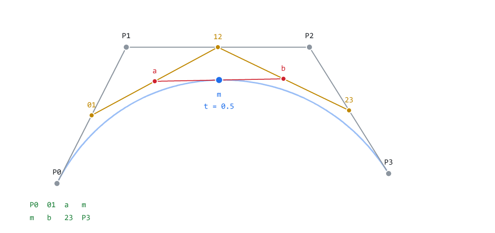
Figure 3. Six averages produce the split point and both halves at once.
Figure 3 is that construction drawn at full size. Grey is the original control polygon P0–P1–P2–P3. Amber is the first level: the three midpoints 01, 12 and 23, joined. Red is the second level: a and b, the midpoints of the amber segments, joined. Blue is where it terminates, at m — and m sits on the curve, not merely near it.
Read the left half straight off the picture: start at P0, then the first amber point 01, then the red point a, then m. The right half is the mirror of that, running m, b, 23, P3. Both halves are exact: they are not approximations of the two pieces of the original curve, they are the two pieces, expressed in the only form the algorithm understands.
Six averages. No powers, no divisions, and the whole thing is numerically stable in the ordinary range of coordinates — which is not a throwaway remark when you are recursing on control points a caller handed you. It is not unconditionally safe: (x0 + x1) * 0.5 can overflow on large finite doubles, because the addition happens before the halving. For UI coordinates this never matters, but a library that accepts arbitrary input should be aware that the midpoint form is stable, not magic.
Here is the recursion in full, which is the function those six lines live in:
//+------------------------------------------------------------------+
//| Adaptive cubic Bézier flattening, by recursive midpoint          |
//| splitting - the De Casteljau algorithm.                          |
//+------------------------------------------------------------------+
void CCairoPath::FlattenCubic(const double x0, const double y0,
                              const double x1, const double y1,
                              const double x2, const double y2,
                              const double x3, const double y3,
                              const int depth)
  {
   const double d1 = DistanceToChord(x1, y1, x0, y0, x3, y3);
   const double d2 = DistanceToChord(x2, y2, x0, y0, x3, y3);

//--- Flat enough, or too deep: emit the chord and stop.
//---
//--- Only the END point is emitted. The start is already in the
//--- array - put there by the MoveTo that opened the contour, by
//--- the LineTo before this curve, or by the previous recursive
//--- call. Emitting both ends would duplicate every interior
//--- vertex: same picture, twice the edges.
   if(depth >= 18 || (d1 + d2) <= CairoFlattenTolerance)
     {
      AddPoint(x3, y3);
      return;
     }

//--- De Casteljau split at t = 0.5: every value here is a midpoint
   const double x01 = (x0  + x1) * 0.5, y01 = (y0  + y1) * 0.5;
   const double x12 = (x1  + x2) * 0.5, y12 = (y1  + y2) * 0.5;
   const double x23 = (x2  + x3) * 0.5, y23 = (y2  + y3) * 0.5;
   const double xa  = (x01 + x12) * 0.5, ya  = (y01 + y12) * 0.5;
   const double xb  = (x12 + x23) * 0.5, yb  = (y12 + y23) * 0.5;
   const double xm  = (xa  + xb) * 0.5, ym  = (ya  + yb) * 0.5;

//--- Left half first, then the right half. THE ORDER MATTERS:
//--- vertices are appended in traversal order, and a contour whose
//--- vertices arrive out of order is not the shape you drew - it
//--- is a self-intersecting one, which the fill rules of Part 5
//--- will shade in ways that are hard to diagnose from a picture.
   FlattenCubic(x0, y0, x01, y01, xa,  ya,  xm, ym, depth + 1);
   FlattenCubic(xm, ym, xb,  yb,  x23, y23, x3, y3, depth + 1);
  }
Four details in there deserve attention, because each one is a decision rather than a formality.
Only x3, y3 is emitted. The start point is not, because it is already in the array — put there by the MoveTo that opened the contour, by the LineTo before this curve, or by the recursive call that just finished. Emitting both ends of every chord would duplicate every interior vertex. The rendered shape would be identical, because a zero-length segment contributes no edge, but the edge list would be twice the size for nothing, and the vertex counts the demo prints would become a lie.
The order matters. Left half first, then right. Vertices are appended in traversal order, and a contour whose vertices arrive out of order is not the shape you drew — it is a self-intersecting version of it. Swap those two lines and the path still fills; it fills as a bow-tie, and the winding rule from Part 5 will shade the crossing region in a way that is genuinely hard to trace back to two transposed statements.
The depth cap is a real guard, not decoration. Each split roughly quarters the deviation, as Figure 2 measured, so an ordinary UI curve finishes in five or six levels. A cap of 18 is far beyond what any sane shape needs, and that is what makes it a useful backstop: it should never fire for normal input, and it always fires when the flatness test cannot terminate on its own. It is not a proof that 18 is unreachable — a pathological input with very large coordinates, a very small tolerance or a deliberately vicious curve can drive the recursion that deep. It also does not make the input valid. What it protects against is input where the flatness test can never succeed — a NaN coordinate, an infinity, a control point that arrived from a division by zero. NaN <= tolerance is false, so the test never passes and the recursion never returns. Without the cap, this becomes infinite recursion inside OnCalculate() or OnTimer(). In the terminal, that can freeze the chart and leave an EA that cannot be removed. With the cap in place, the recursion stops — but it still adds a point, which may itself be NaN or Infinity, and at depth 18 a visibly coarse chord may be emitted regardless of the requested tolerance. The cap bounds the damage; it does not cure the data.
The test is conservative, and that is intentional. d1 + d2 is an upper bound on how far the curve strays from the infinite line through the chord, not a complete measure of the geometric error. The true maximum deviation of a cubic from its chord is bounded by roughly three quarters of the larger of the two distances, so summing them overshoots on purpose. A tolerance of 0.30 px therefore produces a curve that is typically well inside 0.30 px. There is a class of cases the test does not capture by itself: a curve that is collinear with the chord but extends beyond it, or that doubles back along the line, can have d1 = d2 = 0 and still be flattened into a segment that does not cover the original path. Those cases are rare in UI geometry, where curve control points are not usually placed exactly on the chord, but they are real. The test should be read as a conservative bound on perpendicular deviation, not as a proof that a passing curve is indistinguishable from its chord.
Why adaptive beats a fixed segment count
The obvious alternative to all of this is a loop: evaluate the curve at 32 evenly spaced values of t and emit 32 segments. It is simpler, it is what most people write first, and it is worth understanding precisely why it is worse — because "adaptive is better" is the kind of claim that gets repeated without being checked.
It is not that a fixed count is always slower, or always coarser. On any single curve you can pick a count that is neither, and for a known class of shapes at a known scale a fixed count can be sufficient and faster. The problem is that you have to pick it per curve, and the code that calls CurveTo does not know what it is drawing. Adaptive subdivision is the better default because it removes that decision from every caller; it is not a universal theorem about all possible curves.
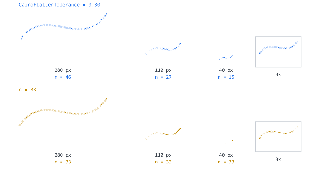
Figure 4. One tolerance across three sizes, and what a fixed count costs.
Figure 4 is that argument made with numbers. The top row is adaptive, the bottom row is the fixed loop, and both rows draw the same curve shape at three sizes: a 280-pixel sweep, a 110-pixel bend and a 40-pixel corner. That is not a contrived spread — it is what a single dashboard contains, between a chart outline and the rounded corner of a button. The boxes on the right are the 40-pixel case again, magnified three times, because at true scale you cannot see where its vertices fall.
Flattened adaptively at one tolerance of 0.30 px, the three curves take 46, 27 and 15 vertices. Each one got what its own size and its own curvature asked for, and no caller had to know anything about any of them.
The fixed loop gives all three of them 33. The 40-pixel corner, which no eye will resolve past about a dozen segments, costs more than twice what it needs and slightly more than the adaptive version spends on a curve seven times its size. Look at the magnified box on the bottom row: the vertices are packed so tightly they overlap into a solid line. Every one of them costs an entry in the edge list, a sort comparison, and a walk through the scanline loop of Part 3.
The waste is the smaller half of the problem. A curve tighter than any of these — a hairpin at the same 280 pixels — would be starved at the same 33 and come out visibly faceted, and there is no single number that fixes both ends of that. Raise the constant to serve the hairpin and every corner radius in the interface pays for it.
The demo makes the distribution visible as well as the count. Panel C draws a path with a tight bend at one end and a nearly straight run at the other, and marks every vertex the flattener produced. They cluster densely in the bend and thin out to almost nothing along the straight part, because the recursion only splits where the chord test fails.
A useful general principle applies here (and in Part 4): let the work follow the difficulty. Uniform effort applied to a non-uniform problem is almost always the wrong trade, and it is usually wrong in both directions at the same time.
The tolerance, and the setting it is not
Config.mqh gains its second value. Here is the whole addition, comment included, because the comment is doing as much work as the line under it:
//+------------------------------------------------------------------+
//| CairoFlattenTolerance                           (added in Part 6)|
//+------------------------------------------------------------------+
double CairoFlattenTolerance = 0.30;
It is a global rather than a #define, for the same reason CairoAaSamples is: quality is something an application legitimately changes at runtime. Full fidelity for a panel that is drawn once and then sits there; draft while the user is dragging something and forty frames a second matter more than a perfect outline. Panel B of the demo does exactly that, saving the value, sweeping it through four settings and restoring it.
The global does have a cost, and it is worth naming: the vertices a path contains depend on a value outside the path. The same CurveTo sequence can produce different vertex arrays depending on when it was called and what the tolerance happened to be. That is acceptable for a UI library, where rebuilding a path and drawing it are practically simultaneous, but it means a path is not a purely self-contained object. Two paths built from identical calls at different moments are not guaranteed to be identical.
Because CairoFlattenTolerance is read in the flatness test, its value should be sane. A negative value, or a NaN, makes (d1 + d2) <= CairoFlattenTolerance false for every piece, so the recursion is driven to the depth cap and every chord is emitted at whatever resolution the cap implies. A very small positive value produces the same effect more slowly, with a sharp rise in the segment count. The library does not currently validate the value; applications that expose it should clamp it to a positive, finite number.
Expressing it in pixels rather than as a segment count is what makes the same constant work across sizes, and that is worth more than it first appears. A four-pixel corner radius gets a handful of segments. A four-hundred-pixel circle gets many. Neither number was guessed by anyone, neither has to be maintained, and the same constant stays correct when a panel is resized. This is not the same as being scale-independent for an already-built path: the path is fixed once it is flattened, and scaling it afterwards scales the facets with it. What the pixel tolerance buys is that the same code that rebuilds a path for a new size gets an appropriately detailed path at that size. This becomes very concrete in Part 7, when rounded rectangles start generating arcs whose radii vary by two orders of magnitude inside a single widget.
It is not the anti-aliasing setting
These two get confused constantly, so let us be explicit about it:
| Setting | Controls |
|---|---|
| CairoFlattenTolerance | how faithful the outline is to the mathematical curve |
| CairoAaSamples | how smoothly that outline is painted |
A curve flattened at 0.30 px still gets perfectly smooth edges, because the rasterizer anti-aliases whatever segments it is handed and has no idea they came from a curve. So if a large circle looks faceted — straight sections meeting at visible corners — raising CairoAaSamples will not help at all. The rasterizer is faithfully painting the coarse outline it was given, and painting it more carefully will not make it a different outline. CairoFlattenTolerance is the dial you want. If a diagonal edge looks stepped rather than faceted, the reverse is true.
Keeping both values in Config.mqh, with that distinction written down next to them, is worth more than any amount of documentation kept elsewhere, because the person who needs it is looking at a picture that is wrong and is about to change something.
One consequence of this addition is worth noting in passing: Path.mqh now reads a tunable, so it gains an include it did not have before.
#ifndef CAIRO5_PATH_MQH
#define CAIRO5_PATH_MQH

//--- FlattenCubic reads CairoFlattenTolerance
#include "Config.mqh"
The two curve verbs
Everything above is machinery. The public surface this part adds is two functions, and both are short, because the flattener is doing the work.
//+------------------------------------------------------------------+
//| CurveTo - a cubic Bézier from the pen, through the control       |
//| points (x1,y1) and (x2,y2), ending at (x3,y3).                   |
//+------------------------------------------------------------------+
void CCairoPath::CurveTo(const double x1, const double y1,
                         const double x2, const double y2,
                         const double x3, const double y3)
  {
   if(!m_has_current)
      MoveTo(m_cur_x, m_cur_y);

   FlattenCubic(m_cur_x, m_cur_y, x1, y1, x2, y2, x3, y3, 0);
  }
The start point is implicit — it is wherever the pen already is. That is why CCairoPath has been tracking m_cur_x and m_cur_y since Part 2, when it looked like a small convenience for LineTo. Four articles later it turns out to be what makes the curve verbs match every other vector API in existence: SVG, PostScript and Cairo all take three points for a cubic and take the fourth from the current position.
The guard on the first line is the same forgiveness LineTo has always shown. m_has_current is a real piece of state, not a guess from the contour count: it is false on a fresh path and false again after Close() lifts the pen. Without the guard, a CurveTo in either of those situations would hand vertices to AddPoint with no contour open to hold them, and they would silently join whatever contour happened to be last. Opening one at the pen's position is what the caller almost certainly meant, and it matches what LineTo does one screen above it in the same file.
The second verb is the quadratic.
//+------------------------------------------------------------------+
//| QuadTo - a quadratic Bézier, with ONE control point.             |
//+------------------------------------------------------------------+
void CCairoPath::QuadTo(const double cx, const double cy,
                        const double x,  const double y)
  {
   const double x1 = m_cur_x + 2.0 / 3.0 * (cx - m_cur_x);
   const double y1 = m_cur_y + 2.0 / 3.0 * (cy - m_cur_y);
   const double x2 = x       + 2.0 / 3.0 * (cx - x);
   const double y2 = y       + 2.0 / 3.0 * (cy - y);

   CurveTo(x1, y1, x2, y2, x, y);
  }
A quadratic Bézier has only one control point rather than two. It matters because TrueType fonts use quadratics exclusively, so any future glyph work will arrive in that form and will need somewhere to go.
We do not write a second flattener. Every quadratic is a cubic, and the conversion is exact:
C1 = P0 + 2/3 * (Q - P0)
C2 = P2 + 2/3 * (Q - P2)
Read that geometrically: each cubic control point sits two thirds of the way from an endpoint towards the single quadratic control point Q. Nothing is approximated here. This is degree elevation, and it is exact for Bézier curves: those two control points describe the same curve as the original single one, point for point, at every value of t. It is not a fit and it is not a close approximation — it is the same curve written down differently.
The payoff is that the library keeps one curve implementation, which means one place for bugs to live instead of two, and one place to optimize if it ever matters. Panel D of the demo verifies the conversion with a visual check: it draws the same curve twice, once through QuadTo in a thick color and once through the hand-converted cubic in a thin color on top. If the conversion were even slightly off, the thick color would show along one side. It does not, and the log confirms that both paths came out with the same 33 vertices. That is a demonstration, not a proof — the proof is the degree-elevation identity above, which is exact by construction. The demo exists to show that the code matches the identity, not to establish the identity.
One subtlety in QuadTo is worth calling out because the guard lives in CurveTo, not here. QuadTo reads m_cur_x and m_cur_y before CurveTo has a chance to guard against a missing current point. If the pen is unset — a fresh path, or one just after Close() — the quadratic control points are computed from whatever the current-position fields hold. CurveTo then opens a contour at that same position, so the curve is drawn from the stale point to the intended endpoint. This matches how LineTo and CurveTo already behave in the same situation, but callers who care should set the start with MoveTo rather than rely on the fallback. The alternative — validating at the top of QuadTo and refusing to draw — would be stricter, and would change the behaviour of the two existing verbs to match it. That change is not part of this article.
That is every line this part adds to the library: one global, one include, and four functions. Raster.mqh, Color.mqh and Surface.mqh were not opened.
The demo
Demo06_Curves.mq5 makes the flattener visible rather than describing it, using the PointX / PointY inspection accessors added in Part 2 for exactly this purpose. Every panel draws a curve and then marks the vertices that were actually produced.
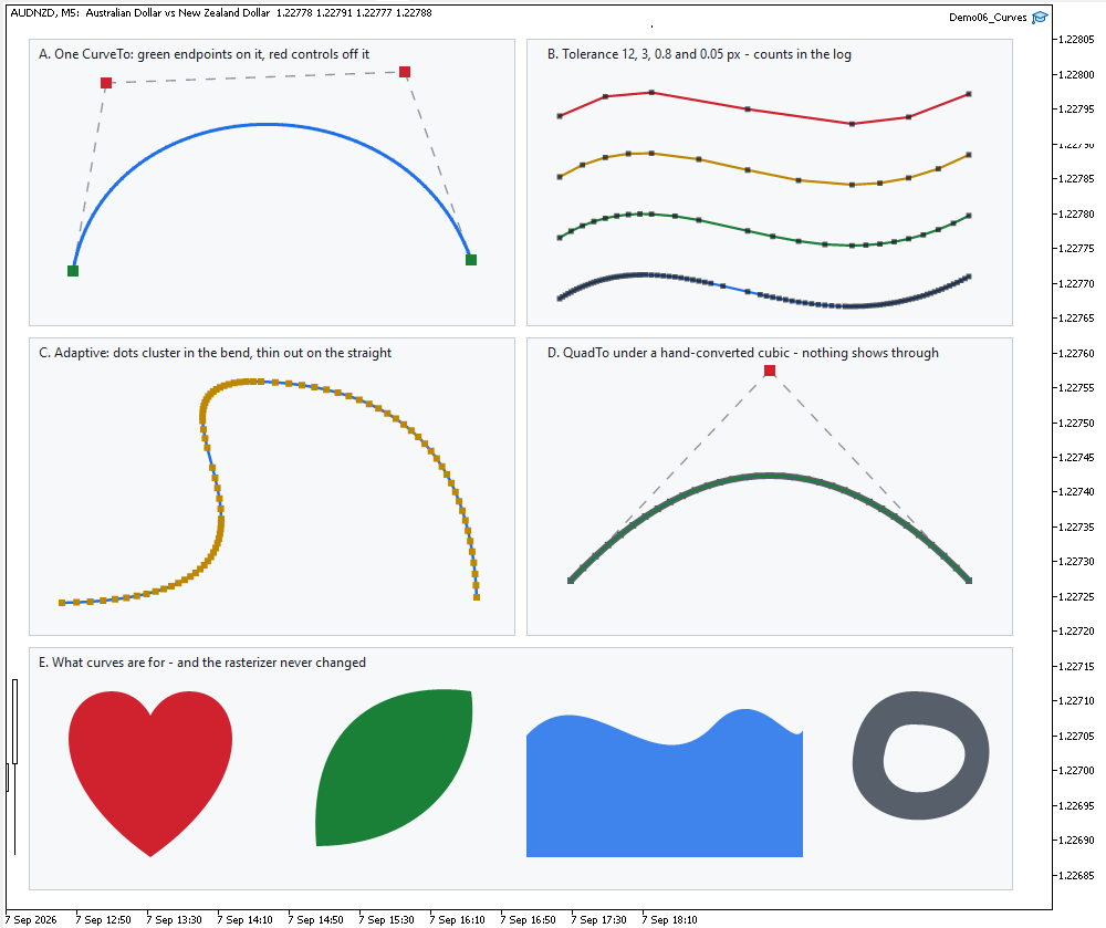
Figure 5. Demo06_Curves on a Black On White chart: five panels of geometry.
- A — anatomy: one CurveTo() with its control polygon, endpoints in green, control points in red. Figure 1, drawn by the engine rather than by the figure script.
//+------------------------------------------------------------------+
//| A. ANATOMY OF A CUBIC BÉZIER                                     |
//+------------------------------------------------------------------+
void PanelAnatomy(const double ox, const double oy)
  {
   Card(ox, oy, 440, 260);

   const double p0x = ox +  40, p0y = oy + 210;
   const double c1x = ox +  70, c1y = oy +  40;
   const double c2x = ox + 340, c2y = oy +  30;
   const double p3x = ox + 400, p3y = oy + 200;

   GuideLine(p0x, p0y, c1x, c1y, C_HULL);
   GuideLine(c1x, c1y, c2x, c2y, C_HULL);
   GuideLine(c2x, c2y, p3x, p3y, C_HULL);

//--- the curve: ONE CurveTo call
   CCairoPath curve;
   curve.MoveTo(p0x, p0y);
   curve.CurveTo(c1x, c1y, c2x, c2y, p3x, p3y);

   StrokeOutline(curve, 3.0, C_CURVE, false);

//--- endpoints: the curve touches these
   CCairoPath ends;
   ends.AddRect(p0x - 5, p0y - 5, 10, 10);
   ends.AddRect(p3x - 5, p3y - 5, 10, 10);
   Fill(ends, C_GREEN);

//--- control points: the curve never touches these
   CCairoPath ctrl;
   ctrl.AddRect(c1x - 5, c1y - 5, 10, 10);
   ctrl.AddRect(c2x - 5, c2y - 5, 10, 10);
   Fill(ctrl, C_CTRL);

   PrintFormat("A. one CurveTo at tolerance %.2f px -> %d vertices",
               CairoFlattenTolerance, curve.PointCount());
  }
- B — the same curve at tolerances of 12, 3, 0.8 and 0.05 pixels. The screen shows the shapes; the log shows the vertex counts, which is what the setting actually controls.
//+------------------------------------------------------------------+
//| B. THE SAME CURVE AT FOUR TOLERANCES                             |
//+------------------------------------------------------------------+
void PanelTolerance(const double ox, const double oy)
  {
   Card(ox, oy, 440, 260);

   const double saved = CairoFlattenTolerance;

   double tolerances[4] = { 12.0, 3.0, 0.8, 0.05 };
   uint   colors[4];

   colors[0] = C_CTRL;
   colors[1] = C_NODE;
   colors[2] = C_GREEN;
   colors[3] = C_CURVE;

   for(int i = 0; i < 4; i++)
     {
      CairoFlattenTolerance = tolerances[i];

      const double y = oy + 40 + i * 55;

      CCairoPath c;
      c.MoveTo(ox +  30, y + 30);
      c.CurveTo(ox + 140, y - 40, ox + 250, y + 90, ox + 400, y + 10);

      StrokeOutline(c, 2.2, colors[i], false);
      MarkVertices(c, 2.4, CairoWithOpacity(DEMO_INK, 0.75));

      PrintFormat("B. tolerance %5.2f px -> %4d vertices",
                  tolerances[i], c.PointCount());
     }

   CairoFlattenTolerance = saved;
  }
- C — adaptive subdivision, with every vertex marked.
//+------------------------------------------------------------------+
//| C. ADAPTIVE SUBDIVISION                                          |
//+------------------------------------------------------------------+
void PanelAdaptive(const double ox, const double oy)
  {
   Card(ox, oy, 440, 270);

   CCairoPath c;
   c.MoveTo(ox +  30, oy + 240);
   c.CurveTo(ox + 320, oy + 235, ox +  55, oy +  35, ox + 210, oy +  40);
   c.CurveTo(ox + 350, oy +  45, ox + 400, oy + 120, ox + 405, oy + 235);

   StrokeOutline(c, 2.5, C_CURVE, false);
   MarkVertices(c, 3.0, C_NODE);

   PrintFormat("C. adaptive: %d vertices, spaced by curvature not by count",
               c.PointCount());
  }
- D — QuadTo() against the hand-converted cubic, drawn on top of each other.
//+------------------------------------------------------------------+
//| D. QUADRATIC vs CUBIC                                            |
//+------------------------------------------------------------------+
void PanelQuadratic(const double ox, const double oy)
  {
   Card(ox, oy, 440, 270);

   const double p0x = ox +  40, p0y = oy + 220;
   const double qx  = ox + 220, qy  = oy +  30;
   const double p2x = ox + 400, p2y = oy + 220;

   GuideLine(p0x, p0y, qx, qy, C_HULL);
   GuideLine(qx, qy, p2x, p2y, C_HULL);

//--- the quadratic
   CCairoPath q;
   q.MoveTo(p0x, p0y);
   q.QuadTo(qx, qy, p2x, p2y);
   StrokeOutline(q, 6.0, C_PURPLE, false);

//--- the same curve, converted by hand, drawn thinner on top
   const double c1x = p0x + 2.0 / 3.0 * (qx - p0x);
   const double c1y = p0y + 2.0 / 3.0 * (qy - p0y);
   const double c2x = p2x + 2.0 / 3.0 * (qx - p2x);
   const double c2y = p2y + 2.0 / 3.0 * (qy - p2y);

   CCairoPath c;
   c.MoveTo(p0x, p0y);
   c.CurveTo(c1x, c1y, c2x, c2y, p2x, p2y);
   StrokeOutline(c, 2.0, C_GREEN, false);

//--- the single control point
   CCairoPath ctrl;
   ctrl.AddRect(qx - 5, qy - 5, 10, 10);
   Fill(ctrl, C_CTRL);

   PrintFormat("D. QuadTo -> %d vertices, hand-converted cubic -> "
               "%d vertices (identical)",
               q.PointCount(), c.PointCount());
  }
- E — what curves are actually for: a heart, a leaf, a wave-topped card, and a curved ring built with the even-odd rule from Part 5.
//+------------------------------------------------------------------+
//| E. WHAT CURVES ARE ACTUALLY FOR                                  |
//+------------------------------------------------------------------+
void PanelShapes(const double ox, const double oy)
  {
   Card(ox, oy, 890, 220);

//--- a heart
   CCairoPath heart;
   heart.MoveTo(ox + 110, oy + 190);
   heart.CurveTo(ox +  10, oy + 120, ox +  25, oy +  40, ox +  75, oy +  40);
   heart.CurveTo(ox + 100, oy +  40, ox + 110, oy +  62, ox + 110, oy +  62);
   heart.CurveTo(ox + 110, oy +  62, ox + 120, oy +  40, ox + 145, oy +  40);
   heart.CurveTo(ox + 195, oy +  40, ox + 210, oy + 120, ox + 110, oy + 190);
   heart.Close();
   Fill(heart, C_CTRL);

//--- a leaf: two curves meeting at two points
   CCairoPath leaf;
   leaf.MoveTo(ox + 260, oy + 180);
   leaf.CurveTo(ox + 250, oy +  60, ox + 330, oy +  30, ox + 400, oy +  40);
   leaf.CurveTo(ox + 410, oy + 110, ox + 360, oy + 180, ox + 260, oy + 180);
   leaf.Close();
   Fill(leaf, C_GREEN);

//--- a card with a wave along its top edge
   CCairoPath wave;
   wave.MoveTo(ox + 450, oy + 190);
   wave.LineTo(ox + 450, oy +  80);
   wave.CurveTo(ox + 505, oy +  20, ox + 565, oy + 130, ox + 620, oy +  70);
   wave.CurveTo(ox + 660, oy +  28, ox + 690, oy +  95, ox + 700, oy +  75);
   wave.LineTo(ox + 700, oy + 190);
   wave.Close();
   Fill(wave, CairoWithOpacity(C_CURVE, 0.85));

//--- a smooth blob, and a ring version of it beside it, to show
//--- curves and fill rules composing
   CCairoPath blob;
   blob.MoveTo(ox + 800, oy +  40);
   blob.CurveTo(ox + 880, oy +  40, ox + 880, oy + 110, ox + 850, oy + 140);
   blob.CurveTo(ox + 820, oy + 170, ox + 740, oy + 160, ox + 745, oy + 100);
   blob.CurveTo(ox + 748, oy +  62, ox + 770, oy +  40, ox + 800, oy +  40);
   blob.Close();

   blob.MoveTo(ox + 800, oy +  70);
   blob.CurveTo(ox + 855, oy +  70, ox + 855, oy + 105, ox + 832, oy + 122);
   blob.CurveTo(ox + 810, oy + 140, ox + 770, oy + 132, ox + 773, oy + 100);
   blob.CurveTo(ox + 776, oy +  80, ox + 782, oy +  70, ox + 800, oy +  70);
   blob.Close();

   Fill(blob, C_PURPLE, CAIRO_EVENODD);
  }
The log is where panel B stops being decorative:
=== Part 6: curves, flattened at tolerance 0.3 px ===
A. one CurveTo at tolerance 0.30 px -> 65 vertices
B. tolerance 12.00 px ->    7 vertices
B. tolerance  3.00 px ->   13 vertices
B. tolerance  0.80 px ->   24 vertices
B. tolerance  0.05 px ->   92 vertices
C. adaptive: 86 vertices, spaced by curvature not by count
D. QuadTo -> 33 vertices, hand-converted cubic -> 33 vertices (identical)
Two things in those numbers are worth more than the picture. The first is the range: the same curve costs 7 vertices or 92 depending on one setting, a factor of thirteen, and the point at which you stop being able to see the difference on your own screen is the tolerance you should actually ship. The second is the last line. QuadTo and the hand-converted cubic produce not "about the same" vertex count but the identical one. That is what the exact conversion from the previous section looks like from the outside; the identity itself was established by the degree-elevation formula, not by the count.
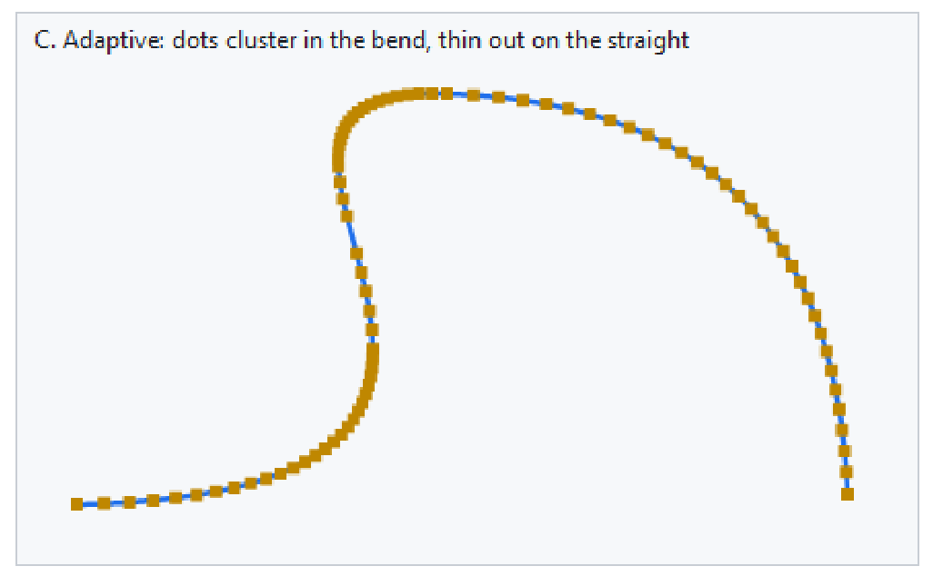
Figure 6. Panel C magnified: vertices crowding the bend, thinning on the run.
Figure 6 is the one to look at closely, and the thing to notice is that no vertex in the sparse region is doing less work than one in the dense region. Each is exactly as necessary as the others; there is simply less curvature to describe out there. That is what "adaptive" means in practice, and it is why the total is smaller than any fixed count that would look as good.
One structural note about the demo: StrokeOutline, MarkVertices and GuideLine are demo helpers, not library code. They are built entirely out of AddThickLine and AddRect — Part 5's tools — because we still have no circles, so a vertex marker is a square and a joint cap is a square. That is mildly ugly under magnification, and it is fixed in the next article.
Project structure
Extract the archive under MQL5/, preserve the folder structure, and compile Demo06_Curves.mq5. No paths need editing.
MQL5/
├── Include/
│   └── CairoG2D/
│       ├── Color.mqh          // the ARGB color type and blending
│       ├── Config.mqh         // CairoAaSamples, now + CairoFlattenTolerance
│       ├── Surface.mqh        // pixel buffer bound to one chart object
│       ├── Path.mqh           // the path and the edges, now + the curves
│       ├── Raster.mqh         // the coverage fill and the fill rule
│       └── DemoTheme.mqh      // the demos' shared palette - NOT library code
└── Experts/
    └── CairoG2D/
        └── Article 06/
└── Demo06_Curves.mq5 // five panels of flattened geometry | # | File | Directory | Holds |
|---|---|---|---|
| 1 | Color.mqh | MQL5/Include/CairoG2D | the ARGB color type and CairoBlendOver |
| 2 | Config.mqh | MQL5/Include/CairoG2D | CairoAaSamples and CairoFlattenTolerance |
| 3 | Surface.mqh | MQL5/Include/CairoG2D | CCairoSurface - pixel buffer to chart bitmap |
| 4 | Path.mqh | MQL5/Include/CairoG2D | the path, the edges, and now the curve verbs |
| 5 | Raster.mqh | MQL5/Include/CairoG2D | CCairoRasterizer - coverage, compositing, fill rule |
| 6 | DemoTheme.mqh | MQL5/Include/CairoG2D | palette, chart setup, captions - not library code |
| 7 | Demo06_Curves.mq5 | MQL5/Experts/CairoG2D/Article 06 | five panels, with the vertices plotted |
| 8 | Cairo-Style Library - Part 06.zip | archive containing all the attached files and their paths relative to the terminal's root folder. |
Two files changed this part, and both only gained. Config.mqh gained CairoFlattenTolerance below CairoAaSamples; nothing above it moved. Path.mqh gained an include, two private functions and two public verbs, all of them appended after LineTo, where the primitive verbs live. Color.mqh, Surface.mqh and Raster.mqh were not touched at all, and the attached include/ folder is exactly what the series has written so far — five files, and nothing from later parts.
What this does not solve, and what is in Part 7
The library can draw curves, and the rasterizer did not change by one line.
That is worth dwelling on, because it was the promise made in Part 1 and it is the entire justification for how this engine is put together. CurveTo flattens into the same vertex arrays that MoveTo and LineTo have filled since Part 2. BuildEdges sees vertices. The rasterizer sees edges. Neither of them has any idea that curves now exist in the library, and neither of them ever will. That is the whole of what this architecture buys: the rasterizer and the filling path stay simple. Operations that need the analytic curve — transformations, dashed strokes, hit testing, length measurement, morphing — are not made easier by this decision and will need their own treatment when they come. Keeping Raster.mqh untouched proves the flatten-before-rasterize boundary is sound for filling; it does not prove the decision is right for everything a path will ever be asked to do.
The algorithm is worth remembering well beyond this project. Recursive subdivision with a cheap, conservative termination test — split until it is good enough, and let the work follow the difficulty — turns up throughout graphics and numerical work once you know to look for it. De Casteljau's method is robust and classical, but it is not the only option: flattening by forward differencing, direct evaluation at adaptive parameter steps, analytic cusp handling and hybrid approaches all exist and are used in production renderers. What recommends De Casteljau here is its simplicity and its locality — each split is a handful of midpoints, no trigonometry, no polynomial coefficients to recompute — not a claim that nothing better has ever been devised.
What the engine still lacks is not power but vocabulary. A Bézier can approximate a circular arc, but only approximately, and you would have to know the magic constant to do it at all. Meanwhile the shapes an interface is actually made of are not general curves: they are arcs, circles, ellipses and rounded rectangles, and no one wants to describe a button corner with four control points.
In Part 7 we build exactly those, and arcs get their own treatment rather than being faked with Béziers. For a circular arc the required segment count can be computed directly, from the geometry, using the sagitta — the height of the bulge between a chord and the arc it spans. One line of trigonometry replaces the whole recursion, and it gives a tight bound on the error rather than a conservative one. The result is still a polyline: the arc is approximated, not stored as an exact circle. What changes is that the approximation error is controlled directly and provably, with a segment count derived from the arc's radius and the tolerance instead of from a chord test.
Then rounded rectangles, with an independent radius per corner, which turns out to be one function that covers cards, tabs, pills, chat bubbles, badges, segmented controls and very nearly everything else a dashboard is built from. Plus the radius clamp that stops a large radius from folding a rectangle into a bow-tie.
After Part 7 the geometry layer is finished, and the only thing left is color.
The project is supported on MQL5 Algo Forge. Each part of this series has its own release, frozen at exactly the code that part explains, so whichever article you are reading, its release is the one to download.
Part 6 is here: https://forge.mql5.io/SandroBegashvil/CairoG2D/releases/tag/part-06
Warning: All rights to these materials are reserved by MetaQuotes Ltd. Copying or reprinting of these materials in whole or in part is prohibited.
This article was written by a user of the site and reflects their personal views. MetaQuotes Ltd is not responsible for the accuracy of the information presented, nor for any consequences resulting from the use of the solutions, strategies or recommendations described.


