Neural Networks in Trading: Recurrent Modeling of Market Micromovements (EV-MGRFlowNet)

Introduction

Today's financial markets resemble a gigantic stream of micro-events — an endless sequence of minute changes, each of which bears the imprint of past transactions and a foreshadowing of future ones. Prices fluctuate, volumes ebb and flow, and orders follow one another at a frequency beyond human perception. Analyzing this stream is as difficult as gauging the direction of the wind during a storm: moments turn into milliseconds, noise drowns out the signal, and traditional methods — designed for static snapshots — lose their ability to perceive motion as a continuous process. It is precisely at this intersection — between the speed of information and the limitations of classical models — that the need arises for a fundamentally new perspective on market dynamics.

In recent years, a similar breakthrough has occurred in a related field — the processing of data from event cameras. Devices that record changes in illumination at each point rather than individual frames have given rise to an entire field of research. In this research, the key focus became not the image itself, but the flow of events over time. Traditional convolutional neural networks proved to be of limited use for analyzing such data. They lacked the sensitivity to the successive microshifts that determine the structure of motion. The response to this challenge was the EV-MGRFlowNet framework, presented in the paper "EV-MGRFlowNet: Motion-Guided Recurrent Network for Unsupervised Event-based Optical Flow with Hybrid Motion-Compensation Loss". The proposed framework is a recurrent model capable of learning without supervision by extracting motion structure directly from the event stream.

The authors of EV-MGRFlowNet proposed an architecture that combines the FERE-Net recurrent encoder, the FGD-Net decoder, and the HMC-Loss hybrid loss function. Rather than being fitted to pre-labeled examples, the network learns on its own to understand how changes are distributed over time and space, aligning successive events based on the principle of motion compensation. At the heart of this idea is the observation that dynamics are self-explanatory. If you estimate motion correctly, the event stream will come together into a logical sequence. Thus, EV-MGRFlowNet does not simply compute the optical flow; rather, it constructs an internal representation of the temporal structure based on causal relationships between micro-events.

This concept has a surprisingly close affinity with financial markets. Market data, especially tick data, is also event-driven by nature. There are no frames here; there is only a continuous stream of basic changes — updates to price, volume, and order imbalances. Each such change conveys local information, but only when viewed in a temporal context does it reveal the true picture of market movements. If we view the market as an event-based scene and the stream of quotes as analogous to optical flow, it becomes possible to apply approaches developed for analyzing image dynamics to understanding a financial video sequence.

Traditional analytical methods — from ARIMA to complex neural networks — make forecasts based on fixed data samples, ignoring the continuity of events. They work with averaged values, thereby stripping away the rich structure of intra-second dynamics. In contrast, the event-driven approach offers a model capable of viewing the market as a living organism, where every movement carries momentum and direction. The recurrent component of the EV-MGRFlowNet framework ensures continuous accumulation of context, allowing the system to perceive not just the current tick, but the trajectory that led to it. The hybrid loss function HMC-Loss enables the model to learn to distinguish true price movements from random fluctuations, which is particularly valuable in the presence of market noise.

Consequently, applying the concepts of EV-MGRFlowNet to the field of financial analysis paves the way for the creation of new generations of models capable of sensing the market. We stop viewing data as a static sequence of numbers and begin to see it as a stream of interactions — as a continuous tapestry of events, where each tick is linked to the previous one and foreshadows the next. In this paradigm, the model’s task is no longer simply to predict the next value in the time series, but to reconstruct the internal motion vector — an analogue of optical flow, but in economic space. This approach allows us not merely to predict future prices, but to understand the direction and pace of market dynamics by identifying consistent patterns in market participants' behavior.

It is important to emphasize that event-driven architecture also offers practical advantages. First, it naturally adapts to irregular time series: unlike standard networks, it does not require a fixed data window; it works with sequences of variable length. Second, unsupervised learning reduces reliance on historical labels, which are almost always subjective in financial problems. Finally, the hybrid loss function allows for the integration of temporal consistency metrics with economic criteria — for example, with an assessment of trend stability or the energy of fluctuations. This makes it possible to train the model on raw data streams without human intervention, which makes the system autonomous and resilient to changes in the market regime.

By viewing financial data as an event-based scene, we gain a new level of insight: not just what happened, but how and why the pattern of movement changed. This is especially important in high-frequency trading, where milliseconds determine the outcome. A model capable of detecting the moment when movement loses coherence (the market’s optical flow breaks down) gains a competitive advantage in identifying transition phases, reversals, and the emergence of new impulses. In this sense, EV-MGRFlowNet becomes a framework for perceiving the market, in which each tick is viewed as an element of dynamic movement.

From a practical standpoint, applying the framework to the financial sector involves adapting its modules to the specific nature of the data. Visual events are replaced by market micro-events, spatial coordinates by financial instrument identifiers and order levels, and the temporal context retains the same continuity. The recurrent encoder generates a representation of local motion patterns; the decoder reconstructs the flow vector — the dynamics of changes in price or imbalance; and the loss function compensates for differences between predicted and actual market behavior. Ultimately, the model learns to understand not individual changes, but their direction and speed — what is intuitively referred to as the market’s rhythm.

In fact, we are dealing with a new analytical paradigm — a shift from post-hoc analysis to perceiving the market as it evolves. This makes the EV-MGRFlowNet framework particularly promising for algorithmic trading, risk management, and predictive liquidity monitoring systems. Where dozens of complex indicators and filters were once required, a single self-adjusting module is now sufficient — one that monitors the market just as the eye tracks movement in space, detecting the direction, acceleration, and stability of the motion flow.

The EV-MGRFlowNet Algorithm

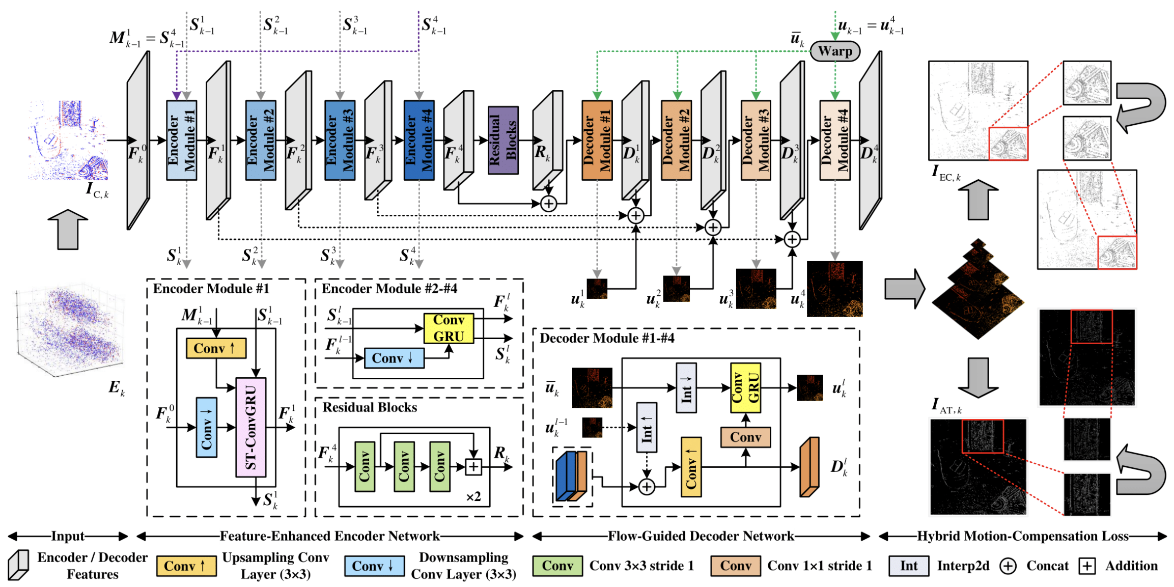
The EV-MGRFlowNet architecture is, at its core, a recurrent encoder-decoder model designed to analyze continuous event streams. It is based on two key components — FERE-Net (Feature-Enhanced Recurrent Encoder) and FGD-Net (Flow-Guided Decoder). The first is responsible for perceiving and accumulating spatiotemporal features, while the second reconstructs and refines motion dynamics across multiple scales.

The model receives an event volume as input, which is then converted into an event count map. In the context of financial markets, this structure can be viewed as analogous to aggregated market micro-events — minor changes in price, volume, or liquidity that occur within short time intervals. This data is processed through FERE-Net, where hidden patterns and temporal relationships are identified. The model’s recurrent nature allows it not only to capture a snapshot of the current state, but also to form a continuous perception of the flow, much like an experienced trader senses the market’s pace and direction by observing subtle changes in the flow of orders.

A key element of the architecture is the use of recurrent ConvGRU and ST-ConvGRU blocks, which ensure the preservation of multilayer hidden states. As a result, the model is capable of detecting even brief spikes and asynchronous shifts in the data — phenomena that, in a market environment, manifest as micro-fluctuations in quotes and transitions between phases of activity.

After the encoding stage, the output features are fed into FGD-Net, where multilevel estimation of directional flow is performed. Here, previously extracted motion information is used to refine new predictions, forming a self-correcting system — a principle that is particularly valuable when dealing with nonlinear and stochastic market processes. Essentially, the model learns to focus not on the price itself, but on its direction and rate of change, thereby forming a picture of market flow.

The final stage of training is based on the hybrid loss function HMC-Loss (Hybrid Motion Compensation Loss), which uses only event data and evaluates reconstruction quality based on the sharpness of temporal and exponential intensity maps. In the context of trading, this can be interpreted as a test of the clarity of market perception: how accurately the model captures actual movement impulses without external training on pre-labeled data.

The motion flow analysis scheme proposed by the authors of the framework uses event cameras — devices capable of recording changes in intensity at each pixel independently and asynchronously. The operating principle of these sensors gives them unique advantages: high temporal resolution and a wide dynamic range. Unlike traditional cameras, which capture images at a constant frame rate, each pixel in an event camera responds only to significant changes in intensity and generates events the moment those changes occur.

Formally, an event ei = (xi, ti, pi) occurs at pixel xi = (xi, yi) when the logarithmic change in intensity exceeds a specified contrast threshold θ at time ti. The event polarity pi ∈ {+1, -1} reflects the direction of the change. This results in a sparse, asynchronous stream of events in three-dimensional coordinates (x, y, t).

A single signal carries very little information, and it is difficult to feed individual events directly into a deep network. Therefore, events are aggregated into short time windows, forming an event representation suitable for processing by a neural network. The event stream is divided into a sequence of event segments Ek spanning fixed time intervals. Each segment is then converted into a convenient representation.

In the authors’ study, the model takes as input an event count map IC,k ∈ R^2*H*W, a representation widely used in event-based vision research. The positive and negative maps IC,+,k and IC,-,k are generated by counting the events at each pixel for the corresponding polarities.

In a financial context, market micro-events — changes in price, volume, or liquidity occurring at each price level of a financial instrument over a short time interval — can be viewed in a similar way. Instead of a visual frame, a market event map is generated, where each pixel represents the number of events at a specific position and within a specific time window. By aggregating micro-events, we obtain a compact yet informative representation that the model can process efficiently to identify patterns and the direction of market movement.

After the event volumes Ek are converted into event count maps IC,k, they are fed into an encoder to extract spatiotemporal features. A key component of the encoder is the convolutional recurrent unit (ConvGRU), which allows the model to take into account the current state of the signal being analyzed and the information accumulated in previous steps. Formally, the hidden state at the current time step (Hk) is computed as a function of the current input (Xk) and the previous hidden state (Hk-1).

This structure allows for the explicit encoding of spatial information while simultaneously capturing temporal dependencies. ConvGRU includes a reset gate (rk) and an update gate (zk), which control the accumulation and updating of the model's memory. These gates provide flexibility in processing event streams, allowing the network to focus on significant changes and forget noisy or irrelevant signals.

The ConvGRU encoder is implemented as a multilayer architecture. In a four-layer implementation, each layer processes the input features and passes the updated hidden states to the next layer. At the same time, each layer accumulates information about events at its own level of resolution. However, the standard ConvGRU architecture has a limitation. The memory of modules at different levels is updated only along the time axis. This means that the lower layers may lose valuable data accumulated by the upper layers — data that is particularly important for capturing small, subtle motion patterns.

To preserve these key spatiotemporal features, the authors of the framework augment FERE-Net with an ST-ConvGRU block. This module extends the capabilities of the standard ConvGRU by creating an additional set of gates for a separate memory (M), which stores information from the upper layer and is combined with the main memory (S) via an output gate (ok) and a 1×1 convolution. This produces the updated feature maps (Fk¹) and hidden state (Sk¹).

The input to the first encoder layer (fE1) consists of three components: the current event map (Fk⁰ = IC,k), the lower layer's hidden state from the previous step (Sk-1¹), and the upper layer's hidden state (Mk-1¹). ST-ConvGRU combines these elements, providing feature enrichment that enables the model to capture local micro-movements and global structural changes in the event stream.

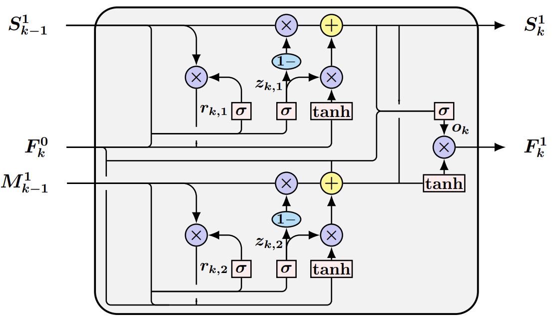
The updated features then pass sequentially through layers (fE2), (fE3), and (fE4), where the standard ConvGRU is used. At each layer, the hidden states from the previous step are integrated with the current features, allowing the model to accumulate information at different levels and capture complex spatiotemporal patterns. The final output features (Fk⁴) are fed into residual blocks (Residual Blocks), which provide additional feature refinement and processing.

These final feature maps (Rk) provide a complete, enriched representation of the event stream, ready for the decoder.

In the context of financial time series, the lower layers of FERE-Net capture instantaneous local fluctuations that can be compared to short-term market impulses. The upper layers accumulate information about broader trends, allowing the model to perceive gradual trends and the overall structure of motion. ST-ConvGRU ensures that key features from different levels are preserved so that the model does not lose information about subtle but significant micro-movements.

Thus, FERE-Net transforms a stream of disparate market events into a structured and enriched representation of market dynamics, making it possible to identify the direction of movement, the intensity of changes, and the stability of market patterns. This serves as the foundation for subsequent decoding and reconstruction of motion flows, enabling the model to predict the market's overall behavior at the micro level.

Optical flow estimation models based on the U-Net architecture rarely use information from previous flows, even though such data can provide effective initialization and additional information to refine the current prediction. The authors of the EV-MGRFlowNet framework address this challenge using a Flow-Guided Decoder Network (FGD-Net), which uses previous flow estimates to improve current predictions.

The first step is to align the successive flow fields (uk-1) and (uk). Since the pixel coordinates on which the previous predictions are based do not match the current ones, the forward warping method is used. Assuming that the flow remains locally constant, we can obtain the aligned flow (û*k) from the previous step (u*k-1).

The decoder consists of four modules fDl… l ∈ (1, 4), enabling multilevel motion flow prediction. At each level, the inputs consist of the intermediate feature maps from the previous decoder layer, the corresponding encoder maps (F5-l,k), and the aligned previous flow (ûk). The output of each module consists of a refined flow (ûlk) and intermediate feature maps (Dlk).

First, the data are combined (concatenated) across channels to form an initial flow prediction (ûlk) and intermediate feature maps (Dlk). Next, a ConvGRU is used to extract motion information from the aligned flow (ûk) and refine the current prediction, generating the final flow (ûlk). At each level, the aligned flow (ûk) is further downsampled to match the size of the feature map.

Thus, the final prediction (û4k) is used as the current flow estimate (uk). In this process, (uk) becomes the preliminary flow for the next decoding step, creating a feedback loop that allows the model to accumulate and refine information about motion dynamics over time.

In the context of financial time series, FGD-Net acts as a mechanism that learns to use information about past market movements to refine current forecasts. Previous estimates, such as historical micro-movements in price or volume, help the model understand trends and predict subsequent changes more accurately, taking into account short-term impulses and accumulated trends.

Thus, the FGD-Net decoder converts the sequence of intermediate features accumulated by FERE-Net into an accurate, multilevel representation of the flow of market micro-movements, where each level corresponds to a distinct scale: from rapid impulses to longer-term trends. This architecture enables the model to perceive the market as a continuous, structured stream of events, allowing it to forecast market dynamics in great detail.

To train EV-MGRFlowNet, the framework’s authors propose a hybrid motion-compensation loss function (Hybrid Motion-Compensation Loss, HMC-Loss), which allows the model to learn without supervision using only event data. This approach is particularly important for financial markets, where there is often no labeled data on correct price movements, and micro-movements occur almost continuously.

The idea behind HMC-Loss is that the model should be able to correctly align events in time, taking into account previous flow predictions. First, the predicted flows (uk ∈ R^2*H*W) are used to shift the event segments under analysis (Ek) to a reference time (t0), forming an aligned volume (E'k). This step can be compared to bringing all minor changes in price and volume onto a single time scale — this allows the model to obtain a consistent picture of what is happening in the market.

Next, the standard loss function LAT (Loss based on Average Timestamp LWE) is used to measure the sharpness of the average timestamp map of events (IAT). LAT evaluates how accurately events are aligned after flow compensation. It is particularly effective at capturing local structural changes and has proven effective in deep learning methods.

However, LAT has a limitation. It does not constrain the geometry of event alignment strictly enough. As a result, the model may generate undesirable motion flows in which individual micro-events remain scattered and the structure of the motion is lost. To address this, the framework’s authors introduce an exponential event count map (LEC, Exponential Count IWE) and a corresponding loss function (LEC). LEC emphasizes pixels without events and amplifies the influence of the global data structure.

Formally, IEC is constructed as follows:

An analogous expression applies to negative events, where α is the saturation coefficient and κ is the bilinear filtering kernel.

The LEC loss function penalizes event scattering and focuses on the global sharpness of the IEC map, which is critical for accurately reproducing the complex structure of micro-movements.

Combining LAT and LEC yields the hybrid HMC-Loss, which simultaneously ensures the accuracy of local temporal patterns and global motion consistency. In addition, a smoothing component Lsmooth is added to minimize flow differences between adjacent pixels and ensure smooth predictions.

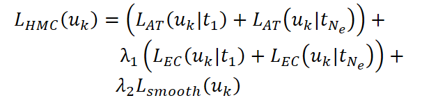
Here, λ1 and λ2 control the balance between local accuracy, global consistency, and flow smoothness. The smoothing term Lsmooth provides gentle, natural regularization.

In the context of financial markets, HMC-Loss acts as an intelligent event aligner. LAT is responsible for accurately reproducing rapid micro-movements in price or volume — analogous to brief market impulses that often precede short-term fluctuations. LEC, in turn, focuses on the global consistency of the flow. This makes it possible to identify trends and the overall structure of market movements. The smoothing component Lsmooth prevents sharp, irrelevant fluctuations in the predicted flow, creating a coherent representation of the microdynamics.

By combining these three elements, EV-MGRFlowNet can effectively learn from real-world market events without labels, while simultaneously capturing local micro-movements and accumulated global trends. As a result, the model can generate detailed and consistent forecasts of market dynamics that account for all levels of movement — from momentary spikes in volume to long-term price trends.

The authors’ visualization of the EV-MGRFlowNet framework is shown below.

Implementation in MQL5

After a detailed examination of the theoretical foundations of EV-MGRFlowNet as proposed by its authors, we will move on to the practical implementation of the framework in the MQL5 environment. Let's start with the key component that can be called the heart of the model — the ST-ConvGRU module. It is this module that ensures the preservation and effective integration of spatiotemporal information, enabling the model to capture local micro-movements and global trends. Implementing ST-ConvGRU requires a careful approach to managing hidden states and layer memory, as well as accurately reproducing convolution operations and recurrent updates.

As the description of the ST-ConvGRU module in the original paper shows, it effectively consists of two parallel ConvGRU modules. We have already implemented a standalone version of ConvGRU in our previous work; however, using multiple modules sequentially results in noticeable delays. This is especially true during the model training phase, when the network repeatedly updates its hidden states.

To minimize the time spent on data processing and training, we need to set up parallel execution of the modules within the OpenCL context. The key point here lies in the structure of the GRU algorithm. If we take a closer look at the operations that update hidden states, we see that most of them are performed element-by-element, with no interdependencies between the various channels.

This means that, regardless of the number of modules, properly organizing the input data allows us to implement them so that the OpenCL program treats multiple modules as one and performs computations in parallel. In this way, we can make effective use of GPU computing resources while preserving the accuracy and correctness of data aggregation and significantly speeding up data analysis and model training.

In practice, this will require structuring the data, carefully designing the channel layout, and using element-wise operations in the OpenCL program to achieve maximum parallelization. This approach will allow us to combine several ConvGRU modules into a single high-performance block, which is particularly important for financial time series with a high event rate and high temporal resolution.

To implement the proposed approach, a new kernel is created in the OpenCL program to process the module's hidden states efficiently in parallel, leveraging the capabilities of the GPU. The kernel takes three arrays as input:

• XH — the concatenated tensor of the required projections of the data being analyzed and the hidden state;
• prev_state — the most recent hidden state;
• outputs — a buffer for storing the results (the module's new hidden state).

__kernel void GRU(__global const float* XH,
                  __global const float* prev_state,
                  __global float* outputs
                 )
  {
   const size_t id = get_global_id(0);
   const size_t d  = get_global_id(1);
   const size_t units = get_global_size(0);
   const size_t dimension = get_global_size(1);

Each work-item is assigned its own indices, which determine the variable and the element of that variable's representation vector that it processes. These indices allow data in linear arrays to be addressed correctly and ensure the proper correspondence between neurons and feature channels.

When accessing the data being analyzed by the GRU, six values corresponding to the standard GRU formula are extracted: the components for the reset gate, the update gate, and the candidate new state, for both the input and recurrent parts. To ensure numerical stability, all extracted values are checked for NaN or infinity.

   const float xz = IsNaNOrInf(XH[RCtoFlat(0, d, 6, dimension, id)], 0);
   const float xr = IsNaNOrInf(XH[RCtoFlat(1, d, 6, dimension, id)], 0);
   const float xh = IsNaNOrInf(XH[RCtoFlat(2, d, 6, dimension, id)], 0);
   const float hz = IsNaNOrInf(XH[RCtoFlat(3, d, 6, dimension, id)], 0);
   const float hr = IsNaNOrInf(XH[RCtoFlat(4, d, 6, dimension, id)], 0);
   const float hh = IsNaNOrInf(XH[RCtoFlat(5, d, 6, dimension, id)], 0);
   const float prev = IsNaNOrInf(prev_state[RCtoFlat(id, d, units, dimension, 0)], 0);

The next step is to compute the GRU elements themselves. First, the reset gate and the update gate are computed using a sigmoid activation function. They determine which parts of the previous state should be retained and which should be replaced.

   float r = fActivation(xr + hr, ActFunc_SIGMOID);
   float z = fActivation(xz + hz, ActFunc_SIGMOID);
   float ht = fActivation(r * hh + xh, ActFunc_TANH);
   float out = (1 - z) * prev + z * ht;

Next, a candidate new hidden state is formed: the reset gate is applied to the recurrent part, and the input contribution, passed through a hyperbolic tangent function for normalization, is added to the result. The final GRU output is then computed as a combination of the previous state and the new candidate, controlled by the value of the update gate.

Finally, this result is written to the array outputs, after its values have been checked once again for validity.

   outputs[RCtoFlat(id, d, units, dimension, 0)] = IsNaNOrInf(out, 0);
  }

The key feature of this implementation is that each operation is performed element-wise; therefore, regardless of the number of ConvGRU modules, their operation can be organized as a single parallel process. An appropriate data structure allows the OpenCL program to process all neurons and channels simultaneously, ensuring high performance and minimal latency.

This approach is particularly effective for processing financial market micro-events, where rapid and accurate aggregation of information from numerous sources is required. The parallel organization of the modules’ operations not only speeds up computations but also ensures that all key features of the hidden states are consistently preserved, which is critical for the network’s continued operation and for training on large time series.

The GRU kernel does not directly train any parameters, since it only performs element-wise computations of hidden states and outputs. However, to train the model correctly, we need to distribute the gradients across all elements of the process. This functionality is implemented by a specialized kernel, GRU_Grad, which computes gradients for each input and hidden state while preserving the parallel processing structure on the GPU.

The kernel takes as input an array XH containing precomputed GRU inputs, an array prev_state containing the previous states of the hidden layer, and an array outputs_gr containing the output gradients. The XH_gr array is used to store the calculated gradients of the inputs.

__kernel void GRU_Grad(__global const float* XH,
                       __global float * XH_gr,
                       __global const float* prev_state,
                       __global const float* outputs_gr
                      )
  {
   const size_t id = get_global_id(0);
   const size_t d  = get_global_id(1);
   const size_t units = get_global_size(0);
   const size_t dimension = get_global_size(1);

Each work-item is assigned its own variable and data dimension indices, which allows for the correct access to elements of multidimensional arrays that have been converted to linear arrays.

   const float xz = IsNaNOrInf(XH[RCtoFlat(0, d, 6, dimension, id)], 0);
   const float xr = IsNaNOrInf(XH[RCtoFlat(1, d, 6, dimension, id)], 0);
   const float xh = IsNaNOrInf(XH[RCtoFlat(2, d, 6, dimension, id)], 0);
   const float hz = IsNaNOrInf(XH[RCtoFlat(3, d, 6, dimension, id)], 0);
   const float hr = IsNaNOrInf(XH[RCtoFlat(4, d, 6, dimension, id)], 0);
   const float hh = IsNaNOrInf(XH[RCtoFlat(5, d, 6, dimension, id)], 0);
   const float prev = IsNaNOrInf(prev_state[RCtoFlat(id, d, units, dimension, 0)], 0);
   const float grad = IsNaNOrInf(outputs_gr[RCtoFloat(id, d, units, dimension, 0)], 0);

The internal components of the GRU — the reset gate, the update gate, and the candidate new state — are computed from the extracted input values and previous states.

   float r = fActivation(xr + hr, ActFunc_SIGMOID);
   float z = fActivation(xz + hz, ActFunc_SIGMOID);
   float ht = fActivation(r * hh + xh, ActFunc_TANH);

Next, backpropagation is performed on these values to compute the gradients for each element: the gradient of the hidden state candidate is multiplied by the update gate; the gradient of the update gate is formed from the difference between the new and previous states; after that, activation-function derivatives are applied to the corresponding input components.

   float ht_grad = IsNaNOrInf(grad * z, 0);
   float z_grad = IsNaNOrInf(grad * (ht - prev), 0);
   float xh_grad = Deactivation(ht_grad, ht, ActFunc_TANH);
   float hh_grad = IsNaNOrInf(xh_grad * r, 0);
   float r_grad = IsNaNOrInf(xh_grad * hh, 0);
   float xz_grad = Deactivation(z_grad, z, ActFunc_SIGMOID);
   float hz_grad = xz_grad;
   float xr_grad = Deactivation(r_grad, r, ActFunc_SIGMOID);
   float hr_gra = xr_grad;

The kernel distributes gradients across all parts of the GRU—the XH input components and the recurrent part of the hidden state. The calculated gradients are stored in the XH_gr array, which has the same structure as the input data, with numerical validity checked using IsNaNOrInf.

   XH_gr[RCtoFlat(0, d, 6, dimension, id)] = IsNaNOrInf(xz_grad, 0);
   XH_gr[RCtoFlat(1, d, 6, dimension, id)] = IsNaNOrInf(xr_grad, 0);
   XH_gr[RCtoFlat(2, d, 6, dimension, id)] = IsNaNOrInf(xh_grad, 0);
   XH_gr[RCtoFlat(3, d, 6, dimension, id)] = IsNaNOrInf(hz_grad, 0);
   XH_gr[RCtoFlat(4, d, 6, dimension, id)] = IsNaNOrInf(hr_grad, 0);
   XH_gr[RCtoFlat(5, d, 6, dimension, id)] = IsNaNOrInf(hh_grad, 0);
  }

This approach preserves computational parallelism on the GPU, ensuring that each element receives its own gradient independently of other work-items.

As a result, GRU_Grad provides the necessary foundation for backpropagation through multiple ConvGRU layers, while maintaining full compatibility with the parallel organization of modules in OpenCL. This is particularly important when working with financial time series, where the speed and accuracy of gradient propagation directly affect the effectiveness of training and the quality of the forecasts generated by the model.

The complete code for the OpenCL program is provided in the attachment.

We've done a lot of work today and deserve a short break to give our brains a rest and take stock of what we've accomplished. In the next article, with renewed energy, we will continue to implement the key approaches proposed by the authors of the EV-MGRFlowNet framework using MQL5, delving deeper into the practical aspects. Step by step, we will move toward the full integration of the proposed algorithms into financial market analysis.

Conclusion

In this article, we examined the architecture of the EV-MGRFlowNet framework in detail and demonstrated how its key components — FERE-Net with the ST-ConvGRU module and FGD-Net — enable the effective modeling of micro-movements. The main advantage of this architecture lies in its ability to fully preserve the spatiotemporal patterns of events, enabling accurate predictions based on even the smallest signals.

The parallel execution of modules within the OpenCL context ensures high performance without sacrificing accuracy, which is critical for processing large streams of market data in real time. The flexibility and scalability of the architecture make it easy to adapt the model to various financial instruments and time intervals, and the use of a hybrid training approach via HMC-Loss ensures robust and accurate reconstruction of event streams.

Links

• EV-MGRFlowNet: Motion-Guided Recurrent Network for Unsupervised Event-Based Optical Flow with Hybrid Motion-Compensation Loss
• Other articles in this series

Programs used in this article

#	Name	Type	Description
1	Study.mq5	Expert Advisor	Expert Advisor for offline model training
2	StudyOnline.mq5	Expert Advisor	Expert Advisor for online model training
3	Test.mq5	Expert Advisor	Expert Advisor for model testing
4	Trajectory.mqh	Class library	Structure describing the system state and model architectures
5	NeuroNet.mqh	Class library	Class library for building a neural network
6	NeuroNet.cl	Library	Code library for an OpenCL program