Practical Modules from Other Languages in MQL5 (Part 08): MATPLOTLIB

MetaTrader 5 — Integration | 9 October 2026, 08:44

130

Omega J Msigwa

“The most important property of a program is whether it accomplishes the intention of its user.”

― C.A.R. Hoare.

Contents

Introduction

Let's face it, data visualization in MQL5 can be challenging. Creating anything beyond a basic visualization often requires an in-depth understanding of how the terminal's chart objects, graphical resources, and canvas system work. While these tools are powerful, they can make the process of creating custom visualizations more technical than it needs to be.

At times, just trying to get a simple plot can feel crude and old-fashioned, especially when compared with the visualization capabilities available in other programming languages. This is understandable considering that MQL5 was primarily designed for financial market analysis and trading automation, not for the fancy-looking GUIs.

image source: pexels.com

When it comes to data visualization, no programming language beats Python. Its large ecosystem and community of data scientists and machine learning developers have produced an enormous number of libraries, frameworks, and tools specifically designed for working with data.

From simple charts to interactive dashboards and advanced statistical visualizations, Python provides developers with a wide range of options.

As we all know, visualization is crucial in getting insights into what your data looks like and in detecting underlying patterns. In MQL5, we usually create custom indicators for the task, which rely on a traditional trading chart environment.

Now, for something that goes beyond a trading chart environment; something lightweight, flexible, good-looking, and relatively easy to use.

This is where Matplotlib becomes useful.

What is Matplotlib?

According to the docs:

Matplotlib is a comprehensive library for creating static, animated, and interactive visualizations in Python. Matplotlib makes easy things easy and hard things possible.

Create publication-quality plots.
Make interactive figures that can zoom, pan, and update.
Customize visual style and layout.
Export to many file formats.
Embed in JupyterLab and Graphical User Interfaces (GUIs).
Use a rich array of third-party packages built on Matplotlib.

See the example below:

import matplotlib.pyplot as plt
import numpy as np

# Data for plotting
t = np.arange(0.0, 2.0, 0.01)
s = 1 + np.sin(2 * np.pi * t)

fig, ax = plt.subplots()
ax.plot(t, s) # t=data on the x axis, s=data on the y-axis

ax.set(xlabel='time (s)', ylabel='voltage (mV)', title='About as simple as it gets, folks')
ax.grid() # sets grid

fig.savefig("test.png") #optional, saves the figure as an image
plt.show() # displays the plot

Results:

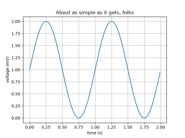
Notice how simple it is? And that's not even the simplest of all examples.

While there are many tools and libraries in Python for visualization purposes, Matplotlib is one of the best. So, in this article, we are going to build a gateway to help us access Matplotlib plots and figures using MQL5 and data provided by the terminal.

Matplotlib in MQL5, The architecture

It all comes down to this flow; below is how the entire project operates:

The architecture

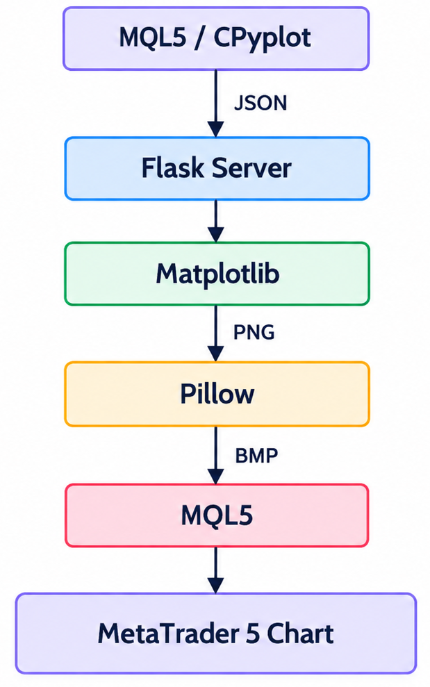
Part 01: MQL5 Client

In MQL5 we are going to have wrapper classes such as CPyplot, which resemble matplotlib.pyplot. Our MQL5 classes will provide methods that resemble those offered in Matplotlib.

For example:

#include <PyMQL5\MatplotLib.mqh>
CPyplot plt;
//+------------------------------------------------------------------+
//| Script program start function                                    |
//+------------------------------------------------------------------+
void OnStart()
  {
//---

   uint total = 100;
   
   vector x = vector::Zeros(100), y;
   y.CopyRates(Symbol(), Period(), COPY_RATES_CLOSE, 0, total);
   
   for (uint i=0; i<total; i++)
      x[i] = i+1;
   
   plt.figure(12, 7.5);
   plt.title(StringFormat("%s, %s close prices",Symbol(),EnumToString(Period())));
   plt.plot(x, y);
   plt.xlabel("Bar index");
   plt.ylabel("close");
   plt.show();
  }

MQL5 functions are responsible for collecting and defining all the information required to generate a plot, such as the data points, title, axis labels, figure dimensions, and grid settings. This information is then serialized into JSON and sent to a local Python Flask server through an HTTP WebRequest().

Part 02: A Flask Server

The Python application provides a lightweight HTTP server using Flask. Its responsibility is deliberately simple: to receive plotting instructions from MQL5 and pass them to a plotting layer.

@app.route("/plot", methods=["POST"])
def plot():

    data = request.get_json()

    # process plotting instructions...
    plot_something(data)
	
    return jsonify({
        "success": True
    })

if __name__ == "__main__":

    print("Starting MQL5 Plot Server...")
    print("Listening on http://127.0.0.1:5000")

    app.run(
        host="127.0.0.1",
        port=5000,
        debug=False
    )

Part 03: Matplotlib

Once the JSON data is received, the plotting layer extracts the required information and uses it when calling appropriate functions.

x = data["x"]
y = data["y"]

fig = Figure(figsize=(12, 7.5))
ax = fig.subplots()

ax.plot(x, y)

ax.set_title(data["title"])
ax.set_xlabel(data["x_label"])
ax.set_ylabel(data["y_label"])
ax.grid(data["grid"])

Part 04: External GUI

The final plot is displayed in a window outside the MetaTrader5 terminal. We'll see how we can plot inside the terminal later on.

Understanding Matplotlib

To mimic Matplotlib interface and syntax in MQL5, we have to get a glimpse on the Matplotlib.

Below is an overview of Matplotlib's figure:

Matplotlib Figure

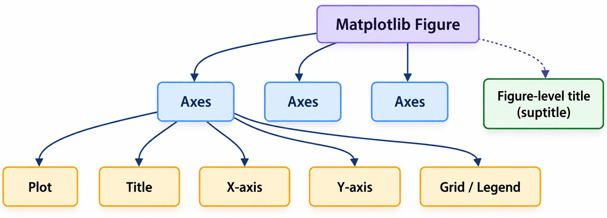
01: Figure

A Figure is the entire Matplotlib window/canvas. Think of it as a piece of paper on which you can draw things.

import matplotlib.pyplot as plt

fig = plt.figure()

This gives you:

matplotlib figure

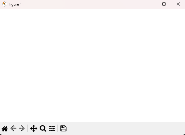
The figure itself isn't necessarily the plot. It is just a container that can have multiple plots.

02: Axes

Axes is the actual plotting area.

For example:

fig = plt.figure()

ax = fig.add_axes([0.1, 0.1, 0.8, 0.8])

Results:

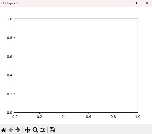
The arguments in a method add_exes() can be confusing.

ax = fig.add_axes([0.1, 0.1, 0.8, 0.8])

Here is what they represent:

[ left, bottom, width, height ]

They represent coordinates on the figure where you want to place the axes. A cleaner way to write this is to use a named argument.

ax = fig.add_axes(
    rect=(
        0.1,  # left
        0.1,  # bottom
        0.8,  # width
        0.8   # height
    )
)

left = 10%
from the left bottom = 10%
from the bottom width = 80% of Figure width
height = 80% of Figure height

Specifying these coordinates can be challenging when working with multiple Axes (plots) in one figure; we'll discuss a better alternative later in this post.

03: Axis

An Axis represents an individual coordinate axis. Not to be confused with Axes; think of this as the X- and Y-axis of a graph.

Axes

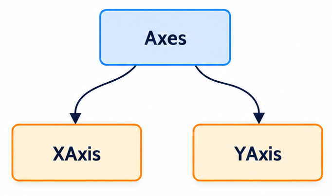
Both X and Y axis objects control things like:

The Figure Class in MQL5

Just like the figure discussed above, the class CFigure class represents a top-level container for a Matplotlib figure in MQL5. Again, in Matplotlib, a figure is the overall drawing surface or window that contains one or more Axes objects.

The class follows the same general idea, but it does not perform the actual rendering itself; it stores the properties and axes that will eventually be translated into JSON and sent to the Python plotting server.

class CFigure
  {
protected:
   double            m_width;
   double            m_height;
   string            m_title;
   string            m_background;
   bool              m_tight_layout;
   bool              m_visible;
   CAxes             m_axes[];

public:
                     CFigure(void);
                    ~CFigure(void);
   
   //--- For adding axes to a figure object
   void              add_axes(CAxes &ax);

   //--- Figure properties
   void              set_size(const double width, const double height);
   double            width(void) const;
   double            height(void) const;

   void              suptitle(const string title);
   string            suptitle(void) const;

   void              facecolor(const string clr);
   string            facecolor(void) const;

   //--- Layout
   void              tight_layout(const bool enable = true);
   bool              tight_layout(void) const;

   //--- Visibility
   void              show(void);
   void              hide(void);
   bool              visible(void) const;

   //--- Figure operations
   void              clear(void);
   void              close(void);
  };

< p> The table represents some of the crucial methods and properties from the above class.

Function	Description
set_size()	Sets dimensions of the figure (width and height, respectively). These values are then stored in the class for the creation of a JSON object we'll discuss later on.
suptitle()	Matplotlib distinguishes between an axes title and a figure-level title. The latter is represented by the so-called "super title" — suptitle().
tight_layout()	This property controls whether the figure should automatically adjust the spacing around its axes. This corresponds to Matplotlib's layout functionality and is particularly useful when a figure contains multiple axes, long labels, or titles that might otherwise overlap.
facecolor()	Controls the background color of the entire figure.
add_axes	Adds axes to the figure by adding the CAxes object (information) to the CFigure.

The Axes class in MQL5

The CAxes class represents an individual plotting area inside a CFigure. This is where most of the actual plotting configuration takes place.

While CFigure controls the overall canvas — its size, background, title, and layout, CAxes controls what is displayed inside that canvas.

This follows the same distinction used by Matplotlib: a figure contains one or more axes, and each axis can have its own title, labels, grid, limits, and plotted data.

class CAxes
  {
protected:
   //--- Title and labels
   string            m_title;
   string            m_xlabel;
   string            m_ylabel;

   //--- Grid
   bool              m_grid;

   //--- Axis limits
   double            m_xmin;
   double            m_xmax;
   double            m_ymin;
   double            m_ymax;

   //--- Autoscaling
   bool              m_autoscale_x;
   bool              m_autoscale_y;

   //--- Axis visibility
   bool              m_xaxis_visible;
   bool              m_yaxis_visible;

   //--- Legend
   bool              m_legend;

public:
                     CAxes(void);
                    ~CAxes(void);

   //--- Plotting
   void              plot(const vector &x, const vector &y);

   //--- Titles and labels
   void              set_title(const string title);
   string            get_title(void) const;

   void              set_xlabel(const string label);
   string            get_xlabel(void) const;

   void              set_ylabel(const string label);
   string            get_ylabel(void) const;

   //--- Grid
   void              grid(const bool enable);
   bool              grid(void) const;

   //--- Limits
   void              set_xlim(const double xmin, const double xmax);
   void              set_ylim(const double ymin, const double ymax);

   double            xmin(void) const;
   double            xmax(void) const;
   double            ymin(void) const;
   double            ymax(void) const;

   //--- Autoscaling
   void              autoscale(const bool enable = true);

   //--- Axis visibility
   void              xaxis_visible(const bool visible = true);
   void              yaxis_visible(const bool visible = true);

   //--- Legend
   void              legend(const bool enable = true);

   //--- Clear
   void              clear(void);

   //--- Set multiple properties
   void              set(
      const string title = NULL,
      const string xlabel = NULL,
      const string ylabel = NULL,
      const double xmin = DBL_MAX,
      const double xmax = DBL_MAX,
      const double ymin = DBL_MAX,
      const double ymax = DBL_MAX
   );
   
   //--- x and y data access
   vector x_values, y_values;
   
  }

Below are short descriptions of some of the functions available in the class.

Function	Description
plot()	Stores the X and Y data that should be plotted. The data is later included in the JSON representation sent to Python, where it is passed to Matplotlib's plotting functions.
set_title()	Sets the title displayed above the axes. This is different from CFigure::suptitle(), which applies a title to the entire figure.
set_xlabel()	Sets the label displayed along the X-axis.
set_ylabel()	Sets the label displayed along the Y-axis.
grid()	Enables or disables the grid displayed behind the plot.
set_xlim()	Explicitly defines the minimum and maximum values displayed on the X-axis.
set_ylim()	Explicitly defines the minimum and maximum values displayed on the Y-axis.
autoscale()	Enables automatic scaling of the axes based on the plotted data.
axis_visible()	Controls whether the X-axis is visible.
yaxis_visible()	Controls whether the Y-axis is visible.
legend()	Enables or disables the legend for the axes.
clear()	Removes the data and resets the axes configuration.
set()	Provides a convenient way of configuring several axes properties with a single function call.

The Pyplot MQL5 class

According to the docs:

matplotlib.pyplot is a collection of functions that make matplotlib work like MATLAB. Each pyplot function makes some change to a figure: e.g., creates a figure, creates a plotting area in a figure, plots some lines in a plotting area, decorates the plot with labels, etc.

Pyplot simplifies the entire plotting process by providing a convenient, state-based interface for creating and customizing plots.

Think of it as a shortcut for quickly visualizing data without having to explicitly manage Figure and Axes objects yourself. It maintains the current figure and plotting state behind the scenes, allowing you to create, configure, and display plots with minimal code.

Instead of requiring the user to explicitly create and manage Figure and Axes objects, Pyplot manages them internally.

Pyplot example in Python:

plt.figure(figsize=(12, 7.5))

plt.plot(x, y)

plt.title("XAUUSD Close Price")
plt.xlabel("Bar Index")
plt.ylabel("Price")
plt.grid(True)

plt.show()

In our corresponding class in MQL5 we maintain a CFigure and a CAxes object internally.

class CPyplot
  {
protected:

   CFigure           m_figure;
   CAxes             m_axes;

   // ....
 };

This is what allows the class to provide a simple interface while still using the more structured CFigure and CAxes underneath.

The relationship in the class looks like this.

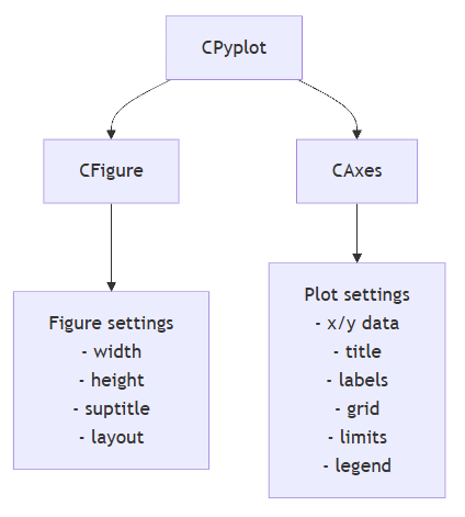
So, when a user calls:

plt.figure(12, 7.5);

CPyplot forwards the values to its internal CFigure object.

m_figure.set_size(width, height);

Similarly, when:

plt.xlabel("Bar Index");

Is called, the value is forwarded to the internal CAxes object.

m_axes.set_xlabel(label);

The CPyplot class does not duplicate the functionality implemented by CFigure and CAxes; instead, it provides a convenient interface for working with them.

The show() Method

The most important method in our CPyplot class is show().

In Matplotlib-Python, pyplot.show() tells Matplotlib to display the current figure.

Unlike the show method offered in Matplotlib-Python, which does the plotting, the one we have in our CPyplot-MQL5 class sends this information to a Python server.

pyplot.mqh

//+------------------------------------------------------------------+
//| Send plot information to Python                                  |
//+------------------------------------------------------------------+
bool CPyplot::show(void)
  {
//--- Figure object
   JSON::Object *figure = new JSON::Object();

   figure
   .setProperty("width",    m_figure.width())
   .setProperty("height",   m_figure.height())
   .setProperty("suptitle", m_figure.suptitle());

//--- X data
   JSON::Array *x = new JSON::Array();

   for(ulong i = 0; i < m_axes.x_values.Size(); i++)
      x.add(m_axes.x_values[i]);

//--- Y data
   JSON::Array *y = new JSON::Array();

   for(ulong i = 0; i < m_axes.y_values.Size(); i++)
      y.add(m_axes.y_values[i]);

//--- X limits
   JSON::Array *xlim = new JSON::Array();

   xlim
   .add(m_axes.xmin())
   .add(m_axes.xmax());

//--- Y limits
   JSON::Array *ylim = new JSON::Array();

   ylim
   .add(m_axes.ymin())
   .add(m_axes.ymax());

//--- Axes object
   JSON::Object *axes = new JSON::Object();

   axes
   .setProperty("title",  m_axes.get_title())
   .setProperty("xlabel", m_axes.get_xlabel())
   .setProperty("ylabel", m_axes.get_ylabel())
   .setProperty("grid",   m_axes.grid())
   .setProperty("xlim",   xlim)
   .setProperty("ylim",   ylim)
   .setProperty("x",      x)
   .setProperty("y",      y);

//--- Root object
   JSON::Object *json = new JSON::Object();

   json
   .setProperty("figure", figure)
   .setProperty("axes",   axes);

//--- Convert to string
   string data = json.toString();

   if(MQLInfoInteger(MQL_DEBUG))
     {
      Print("Plot JSON:");
      Print(data);
     }

//--- delete object pointers

   del_valid_ptr(figure)
   del_valid_ptr(x)
   del_valid_ptr(y)
   del_valid_ptr(xlim)
   del_valid_ptr(ylim)
   del_valid_ptr(axes)
   del_valid_ptr(json)

//--- Send to Flask

   CResponse response = m_session.post(m_url+m_url_suffix, data);
   return response.ok;
  }

The function builds a JSON object based on all the essential information provided in both CFigure and CAxes.

Starting with figure information that includes width, height, and suptitle:

JSON::Object *figure = new JSON::Object();

figure
   .setProperty("width",    m_figure.width())
   .setProperty("height",   m_figure.height())
   .setProperty("suptitle", m_figure.suptitle());

X and Y vectors are then converted into JSON arrays.

JSON::Array *x = new JSON::Array();

for(ulong i = 0; i < m_axes.x_values.Size(); i++)
   x.add(m_axes.x_values[i]);

JSON::Array *y = new JSON::Array();

for(ulong i = 0; i < m_axes.y_values.Size(); i++)
   y.add(m_axes.y_values[i]);

Axes limits are passed as an array of two items (x min and x max) for the x-axis (y min and y max) for the y-axis.

//--- X limits
   JSON::Array *xlim = new JSON::Array();

   xlim
   .add(m_axes.xmin())
   .add(m_axes.xmax());

//--- Y limits
   JSON::Array *ylim = new JSON::Array();

   ylim
   .add(m_axes.ymin())
   .add(m_axes.ymax());

We then assemble the axes object.

JSON::Object *axes = new JSON::Object();

axes
   .setProperty("title",  m_axes.get_title())
   .setProperty("xlabel", m_axes.get_xlabel())
   .setProperty("ylabel", m_axes.get_ylabel())
   .setProperty("grid",   m_axes.grid())
   .setProperty("xlim",   xlim)
   .setProperty("ylim",   ylim)
   .setProperty("x",      x)
   .setProperty("y",      y);

Finally, we assemble the figure object and axes into a single/larger JSON object.

//--- Root object
   JSON::Object *json = new JSON::Object();

   json
   .setProperty("figure", figure)
   .setProperty("axes",   axes);

All the collected information in a JSON object is then sent to a local Python server for plotting.

   CResponse response = m_session.post(m_url + m_url_suffix, data);

Shortly after, the JSON object is converted to a string.

string data = json.toString();

Notice, we are using the Python-like Web request module discussed in this article, for web functionality.

Matplotlib Syntax in MQL5

With everything in place, let us attempt to plot the closing prices on a line plot in Matplotlib from our MQL5 code.

Matplotlib Test.mq5

#include <PyMQL5\MatplotLib\pyplot.mqh>
CPyplot plt;
//+------------------------------------------------------------------+
//| Script program start function                                    |
//+------------------------------------------------------------------+
void OnStart()
  {
//--- collect x and y data to plot

   uint total = 100;
   
   vector x = vector::Zeros(100), y;
   y.CopyRates(Symbol(), Period(), COPY_RATES_CLOSE, 0, total); 
   
   for (uint i=0; i<total; i++)
      x[i] = i+1;

//---

   plt.figure(12, 7.5);
   plt.title(StringFormat("%s, %s close prices",Symbol(),EnumToString(Period())));
   plt.plot(x, y);
   plt.xlabel("Bar index");
   plt.ylabel("close");
   plt.show();
  }

Cool?

However, for this to work, we need a local server that listens to our actions in MQL5, accepts plotting instructions, and acts on them by calling the respective functions to create and run Matplotlib.

First things first, add the local host URL to the list of allowed URLs in your MetaTrader 5 terminal.

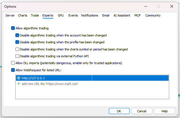
Matplotlib's Python Server

Inside a Python script, we import the necessary modules:

main.py

from flask import Flask, request, jsonify
import utils
import numpy as np
import matplotlib.pyplot as plt

We then initialize the Flask app instance.

app = Flask(__name__)

At the moment, the code we have only implemented the code for drawing a line plot inside CAxes in our MQL5 code:

//+------------------------------------------------------------------+
//| Line plot                                                        |
//+------------------------------------------------------------------+
void CAxes::plot(const vector &x, const vector &y, string c=NULL)
  {
   this.x_values = x;
   this.y_values = y;

   set_plot_type("lineplot");
  }

We create its route in the Flask app.

@app.route("/lineplot", methods=["POST"])
def lineplot():

Inside the function lineplot(), we receive JSON data and extract all plot information from it as provided in MQL5 (to prevent pointless failures, we assign default values when some values are not provided).

def lineplot():

    data = request.get_json()

    print(f"Received plot data: {data}")

    # check if all crucial keys are present in the data

    try:
        figure = data["figure"] # Figure data
        axes = data["axes"] # Axes information

        x = axes["x"]
        y = axes["y"]

    except KeyError as e:

        print(f"Missing key in data: {e}")
        return None

    # extract figure and axes properties with default values if not provided
    
    width = figure.get("width", 6.4)
    height = figure.get("height", 4.8)
    suptitle = figure.get("suptitle", "")

    title = axes.get("title", "")
    x_label = axes.get("xlabel", "x")
    y_label = axes.get("ylabel", "y")
    grid = axes.get("grid", True)

    xlim = axes.get("xlim", None)
    ylim = axes.get("ylim", None)

Finally, we create a plot based on the provided information.

    # Create Figure and Axes
    fig, ax = plt.subplots(figsize=(width, height))

    # Plot
    ax.plot(x, y)

    # Axes properties

    ax.set_title(title)
    ax.set_xlabel(x_label)
    ax.set_ylabel(y_label)

    ax.grid(grid)

    # Apply X limits only when explicitly specified
    if (
        xlim is not None
        and xlim != [0.0, 1.0]
        and not np.isinf(xlim).any()
    ):
        ax.set_xlim(*xlim)

    # Apply Y limits only when explicitly specified
    if (
        ylim is not None
        and ylim != [0.0, 1.0]
        and not np.isinf(ylim).any()
    ):
        ax.set_ylim(*ylim)

    if suptitle:
        fig.suptitle(suptitle)
        
    plt.show() #display the plot

    return jsonify({
        "success": True
    })

Getting the server up and running:

if __name__ == "__main__":

    print("Starting MQL5 Plot Server...")
    print("Listening on http://127.0.0.1:5000")
    
    app.run(
        host="127.0.0.1",
        port=5000,
        debug=True,
        use_reloader=False
    )

Running the script will get the server up and running.

Received JSON data looks like this:

{
    "figure": {
        "width": 12.0,
        "height": 7.5,
        "suptitle": "XAUUSD, PERIOD_M15 close prices"
    },
    "axes": {
        "title": "",
        "xlabel": "Bar index",
        "ylabel": "close",
        "grid": false,
        "xlim": [
            0.0,
            1.0
        ],
        "ylim": [
            0.0,
            1.0
        ],
        "x": [
            1.0,
            2.0,
            3.0,
            4.0,
            5.0,
            6.0,
            7.0,
        ...
        ],
        "y": [
            4346.89,
            4351.75,
            4351.41,
            4350.22,
            4350.41,
            4351.75,
            4349.42,
        ...
        ]
    }
}

Working Different Plot Types

The CPyplot class does not need to use a single endpoint for every type of plot. Instead, the plotting method can determine the type of visualization being requested and assign the appropriate URL suffix.

For example, the plot() method is currently intended for a line plot.

//+------------------------------------------------------------------+
//| Sets X and Y values and the url suffix according to the plot type|
//+------------------------------------------------------------------+
void CPyplot::plot(const vector &x, const vector &y)
  {
   this.m_axes.plot(x, y);

   m_url_suffix = "/" + this.m_axes.plot_type();
  }

//+------------------------------------------------------------------+
//| Line plot                                                        |
//+------------------------------------------------------------------+
void CAxes::plot(const vector &x, const vector &y)
  {
   this.x_values = x;
   this.y_values = y;

   set_plot_type("lineplot");
  }

This approach becomes particularly useful because Matplotlib supports many different types of visualizations, each of which may require different data and plotting parameters.

The below table has some visualization techniques and plot types offered in Python-Matplotlib.

Plot type	Purpose	Example
Line plot.	Shows trends or changes in values, particularly across time or an ordered sequence.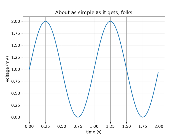
Scatter plot	Displays individual observations as points, making relationships, clusters, and outliers easier to identify.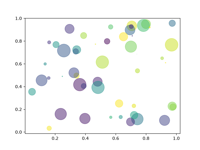
Bar plot	Compares values across discrete categories.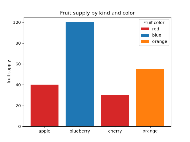
Histogram	Shows the distribution of numerical data by grouping values into bins.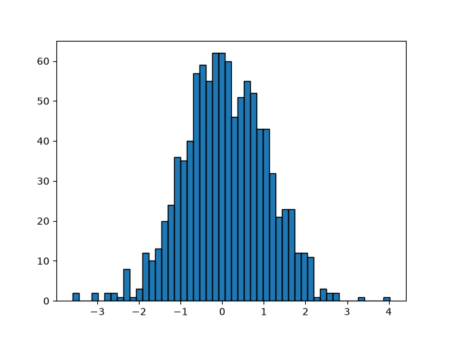
Box plot	Summarizes the distribution of data using quartiles, median, and potential outliers.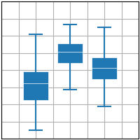
Pie chart	Represents proportions or percentages of a whole.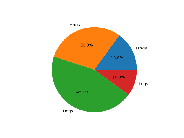
Area plot	Similar to a line plot but fills the area beneath the curve to emphasize magnitude.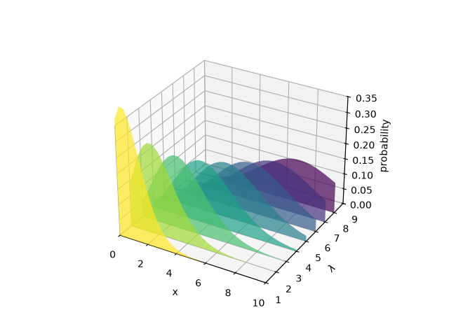
Heatmap	Represents values using a matrix of colors, which is useful for correlations and other two-dimensional data.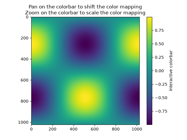

Just like in Python-Matplotlib, we are going to have a separate function for each plot in CAxes and CPyplot.

For example:

plt.plot(x, y);        // Line plot
plt.scatter(x, y);     // Scatter plot
plt.bar(x, y);         // Bar plot
plt.hist(x);           // Histogram

Meanwhile, in the Python server, we have to create different routes for every plot and their individual instructions.

@app.route("/lineplot", methods=["POST"])
def lineplot():
    ...


@app.route("/scatter", methods=["POST"])
def scatter():
    ...


@app.route("/bar", methods=["POST"])
def bar():
    ...


@app.route("/histogram", methods=["POST"])
def histogram():
    ...

The Problem with Matplotlib's GUI

While the current server-based approach works, there is an important limitation when using Matplotlib's interactive GUI.

If a Matplotlib figure is created and displayed directly inside a Flask route, you may see warnings such as:

c:\Users\omega\OneDrive\mql5 articles\Python Modules Series\Matplotlib\main.py:44: UserWarning: Starting a Matplotlib GUI outside of the main thread will likely fail.
  fig, ax = plt.subplots(figsize=(width, height))
c:\Users\omega\OneDrive\mql5 articles\Python Modules Series\Matplotlib\main.py:77: UserWarning: Starting a Matplotlib GUI outside of the main thread will likely fail.
  plt.show() #display the plot

This happens because Matplotlib's GUI is designed to run on the main thread, while the current approach runs it in a background server thread. As a result, creating or displaying a figure directly from the Flask request handler can lead to warnings, plots that do not appear, or an unresponsive GUI depending on the Matplotlib backend and operating system.

There are several workarounds for this issue, including:

Returning a generated plot to MQL5/MetaTrader5 and plotting it there through HTTP.
Not plotting at all, only generating a figure and saving it as PNG/SVG.
Displaying the plot in a web browser.

Displaying Matplotlib Plots in MetaTrader 5

To display plots in the terminal, the Python server must return the generated figure as raw bytes. We update the route to return an image payload.

from flask import Flask, request, jsonify, send_file
import numpy as np

import matplotlib
matplotlib.use("Agg")  # Use a non-interactive backend for Flask

import matplotlib.pyplot as plt
import utils

app = Flask(__name__)

@app.route("/lineplot", methods=["POST"])
def lineplot():
    """Creates a line plot based on the JSON data received in the POST request.

    Returns:
        Optional[None]: A figure object if successful, None if there was an error
    """
    
    data = request.get_json()

    # print(f"Received plot data: {data}")

    # check if all crucial keys are present in the data
    try:
        figure = data["figure"] # Figure data
        axes = data["axes"] # Axes information

        x = axes["x"]
        y = axes["y"]

    except KeyError as e:

        print(f"Missing key in data: {e}")
        return None

    # extract figure and axes properties with default values if not provided

    width = figure.get("width", 6.4)
    height = figure.get("height", 4.8)
    suptitle = figure.get("suptitle", "")

    title = axes.get("title", "")
    x_label = axes.get("xlabel", "x")
    y_label = axes.get("ylabel", "y")
    grid = axes.get("grid", True)

    xlim = axes.get("xlim", None)
    ylim = axes.get("ylim", None)

    # Create Figure and Axes
    fig, ax = plt.subplots(figsize=(width, height))

    # Plot
    ax.plot(x, y)

    # Axes properties

    ax.set_title(title)
    ax.set_xlabel(x_label)
    ax.set_ylabel(y_label)

    ax.grid(grid)

    # Apply X limits only when explicitly specified
    if (
        xlim is not None
        and xlim != [0.0, 1.0]
        and not np.isinf(xlim).any()
    ):
        ax.set_xlim(*xlim)

    # Apply Y limits only when explicitly specified
    if (
        ylim is not None
        and ylim != [0.0, 1.0]
        and not np.isinf(ylim).any()
    ):
        ax.set_ylim(*ylim)

    if suptitle:
        fig.suptitle(suptitle)

    # convert the figure to BMP
    bmp = utils.figure_to_bmp(fig)
    
    return bmp, 200, {
        "Content-Type": "image/bmp"
    }

This time, we explicitly prevent Matplotlib from displaying any sort of figure in the first place.

matplotlib.use("Agg")  # Use a non-interactive backend for Flask

MetaTrader 5 can display BITMAP images using OBJ_BITMAP_LABEL, so the server should convert the figure to a bitmap, return the raw bytes, and MQL5 should fetch them via HTTP.

    bmp = utils.figure_to_bmp(fig)
    
    return bmp, 200, {
        "Content-Type": "image/bmp"
    }

utils.py.

import io
from PIL import Image

def figure_to_bmp(fig):
    """Converts a Matplotlib figure to BMP format.
    
    Parameters:
        fig (matplotlib.figure.Figure): The Matplotlib figure to convert.
    
    Returns:
        bytes: The BMP image data.
    """
    
    # First render the Matplotlib figure as PNG
    png_buffer = io.BytesIO()

    fig.savefig(
        png_buffer,
        format="png",
        bbox_inches="tight"
    )

    png_buffer.seek(0)

    # Open PNG with Pillow
    image = Image.open(png_buffer)

    # BMP does not support RGBA in the same way, so convert it
    image = image.convert("RGB")

    # Convert to BMP
    bmp_buffer = io.BytesIO()

    image.save(
        bmp_buffer,
        format="BMP"
    )

    return bmp_buffer.getvalue()

We also adapt the function for sending plotting commands in MQL5 to return contents returned by the server; in this case, bytes of an image.

//+------------------------------------------------------------------+
//| Sends plot information to Python                                 |
//+------------------------------------------------------------------+
bool CPyplot::show(uchar &res_fig[])
  {
//--- Figure object
   ...
   ...
   ...

//--- Send to Flask

   CResponse response = m_session.post(m_url + m_url_suffix, data);
   ArrayCopy(res_fig, response.content);

   return response.ok;
  }

To test if this works, let us save bytes received from a server to a BITMAP file (download the BITMAP image).

//+------------------------------------------------------------------+
//| Saves image data from a character array to a file.               |
//|                                                                  |
//| Parameters:                                                      |
//|   fig      - Array containing the raw binary image data.         |
//|   filename - Destination filename, relative to the MQL5          |
//|              file sandbox.                                       |
//|                                                                  |
//| Returns:                                                         |
//|   true  - If the file was successfully created and written.      |
//|   false - If the file could not be opened for writing.           |
//+------------------------------------------------------------------+
bool CPyplot::save_fig(uchar &fig[], string filename)
  {
   int handle = FileOpen(filename, FILE_WRITE | FILE_BIN);
   if(handle == INVALID_HANDLE)
     {
      printf("Failed to create %s", filename);
      return false;
     }

   FileWriteArray(handle, fig, 0, ArraySize(fig));
   FileClose(handle);
   return true;
  }

Example usage:

#include <PyMQL5\MatplotLib\pyplot.mqh>
CPyplot plt;
//+------------------------------------------------------------------+
//| Script program start function                                    |
//+------------------------------------------------------------------+
void OnStart()
  {
//--- collect x and y data to plot

   uint total = 100;

   vector x = vector::Zeros(100), y;
   y.CopyRates(Symbol(), Period(), COPY_RATES_CLOSE, 0, total);

   for(uint i = 0; i < total; i++)
      x[i] = i + 1;

//---

   plt.figure(12, 7.5);
   plt.title(StringFormat("%s, %s close prices", Symbol(), EnumToString(Period())));
   plt.plot(x, y);
   plt.xlabel("Bar index");
   plt.ylabel("close");

   uchar image[];
   plt.show(image);

//--- saving the image to Files
   string f = StringFormat("Matplotlib\\%d.bmp", GetTickCount());
   plt.save_fig(image, f);
  }

The outcome is the creation of a BMP image of a figure:

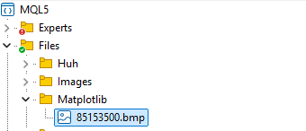
In Windows explorer:

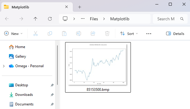
After receiving the image from the server and saving it in the MetaTrader 5 data directory, the terminal can load the same file and display it as a bitmap label.

//+------------------------------------------------------------------+
//|                                                                  |
//| The function creates an OBJ_BITMAP_LABEL graphical object and    |
//| assigns the specified image file to both its ON and OFF states.  |
//| If an object with the same name already exists, it is removed    |
//| before the new bitmap object is created.                         |
//|                                                                  |
//| Parameters:                                                      |
//|   name      - Name of the bitmap object on the chart.            |
//|   file_name - Path to the bitmap image file relative to the      |
//|               MQL5 file sandbox.                                 |
//|                                                                  |
//| Returns:                                                         |
//|   true  - If the bitmap object was successfully created and the  |
//|           image was loaded.                                      |
//|   false - If the object could not be created or the image could  |
//|           not be loaded.                                         |
//|                                                                  |
//| Notes:                                                           |
//|   The bitmap is positioned 30 pixels from the upper-left corner  |
//|   of the chart and displayed in the foreground. The object is    |
//|   selectable but hidden from the chart's object list.            |
//+------------------------------------------------------------------+
bool CPyplot::display_image(const string name, const string file_name)
  {
//--- Remove existing object if it exists
   if(ObjectFind(0, name) >= 0)
      ObjectDelete(0, name);

//--- Create bitmap label
   ResetLastError();

   if(!ObjectCreate(0, name, OBJ_BITMAP_LABEL, 0, 0, 0))
     {
      Print(__FUNCTION__, ": failed to create Bitmap Label! Error = ", GetLastError());
      return false;
     }

//--- Set image for ON state
   ResetLastError();

   if(!ObjectSetString(0, name, OBJPROP_BMPFILE, 0, file_name))
     {
      Print(__FUNCTION__, ": failed to load image! File = ", file_name, " Error = ", GetLastError());
      ObjectDelete(0, name);

      return false;
     }

//--- Image for OFF state
   ResetLastError();

   if(!ObjectSetString(0,name,OBJPROP_BMPFILE,1,file_name))
     {
      Print(__FUNCTION__,": failed to load OFF image! ",file_name," Error = ",GetLastError());
      ObjectDelete(0, name);
      return false;
     }

//--- Position
   ObjectSetInteger(0, name, OBJPROP_XDISTANCE, 30);
   ObjectSetInteger(0, name, OBJPROP_YDISTANCE, 30);

//--- Anchor to upper-left corner
   ObjectSetInteger(0, name, OBJPROP_CORNER, CORNER_LEFT_UPPER);
   ObjectSetInteger(0, name, OBJPROP_ANCHOR, ANCHOR_LEFT_UPPER);

//--- Display in foreground
   ObjectSetInteger(0, name, OBJPROP_BACK, false);

//--- allow user to move it
   ObjectSetInteger(0, name, OBJPROP_SELECTABLE, true);
   ObjectSetInteger(0, name, OBJPROP_SELECTED, true);

//--- Hide from object list
   ObjectSetInteger(0, name, OBJPROP_HIDDEN, true);
   ChartRedraw();

   return true;
  }

Putting it all together!

We call both save_fig() and display_image() inside the show() method, one after the other, to save and display the saved image, respectively.

The show() method now looks like this:

//+------------------------------------------------------------------+
//| Sends plot information to Python                                 |
//+------------------------------------------------------------------+
bool CPyplot::show(void)
  {
//--- Figure object
   JSON::Object *figure = new JSON::Object();

   figure
   .setProperty("width",    m_figure.width())
   .setProperty("height",   m_figure.height())
   .setProperty("suptitle", m_figure.suptitle());

//--- X data
   JSON::Array *x = new JSON::Array();

   for(ulong i = 0; i < m_axes.x_values.Size(); i++)
      x.add(m_axes.x_values[i]);

//--- Y data
   JSON::Array *y = new JSON::Array();

   for(ulong i = 0; i < m_axes.y_values.Size(); i++)
      y.add(m_axes.y_values[i]);

//--- X limits
   JSON::Array *xlim = new JSON::Array();

   xlim
   .add(m_axes.xmin())
   .add(m_axes.xmax());

//--- Y limits
   JSON::Array *ylim = new JSON::Array();

   ylim
   .add(m_axes.ymin())
   .add(m_axes.ymax());

//--- Axes object
   JSON::Object *axes = new JSON::Object();

   axes
   .setProperty("title",  m_axes.get_title())
   .setProperty("xlabel", m_axes.get_xlabel())
   .setProperty("ylabel", m_axes.get_ylabel())
   .setProperty("grid",   m_axes.grid())
   .setProperty("xlim",   xlim)
   .setProperty("ylim",   ylim)
   .setProperty("x",      x)
   .setProperty("y",      y);

//--- Root object
   JSON::Object *json = new JSON::Object();

   json
   .setProperty("figure", figure)
   .setProperty("axes",   axes);

//--- Convert to string
   string data = json.toString();

//if(MQLInfoInteger(MQL_DEBUG))
//   Print("Plot JSON:\n", data);

//--- delete object pointers

   del_valid_ptr(figure)
   del_valid_ptr(x)
   del_valid_ptr(y)
   del_valid_ptr(xlim)
   del_valid_ptr(ylim)
   del_valid_ptr(axes)
   del_valid_ptr(json)

//--- Send to Flask

   CResponse response = m_session.post(m_url + m_url_suffix, data);
   
//--- saving the figure

   string file_name = StringFormat("Matplotlib\\%d.bmp", GetTickCount());
   save_fig(response.content, file_name);

//--- Since bitmap files are searched from the MQL5 parent folder we specify the subfolder '\\Files\\' to the name

   string rel_file_name = "\\Files\\" + file_name; 
   display_image("plot", rel_file_name);
   
   return response.ok;
  }

Example script:

#include <PyMQL5\MatplotLib\pyplot.mqh>
CPyplot plt;
//+------------------------------------------------------------------+
//| Script program start function                                    |
//+------------------------------------------------------------------+
void OnStart()
  {
//--- collect x and y data to plot

   uint total = 100;

   vector x = vector::Zeros(100), y;
   y.CopyRates(Symbol(), Period(), COPY_RATES_CLOSE, 0, total);

   for(uint i = 0; i < total; i++)
      x[i] = i + 1;

//---

   plt.figure(12, 7.5);
   plt.title(StringFormat("%s, %s close prices", Symbol(), EnumToString(Period())));
   plt.plot(x, y);
   plt.xlabel("Bar index");
   plt.ylabel("close");

   plt.show();
   DebugBreak();
  }

Results:

Final Thoughts

With the architecture now in place, we have a solid foundation for bringing Matplotlib-style plotting into MQL5. Rather than trying to reproduce Matplotlib itself inside MQL5 as we usually do in this series, we have created a library that communicates with Matplotlib in Python and gets the job done with a few extra steps.

The library provides a familiar interface for defining figures, axes, plot data, and visual properties, while the actual rendering is delegated to Python and Matplotlib.

In this article, we have seen how Matplotlib operates on a basic level, including figures, axes, and the Pyplot submodule. Since Matplotlib is an extensive library with a large number of plot types, configuration options, styling parameters, and specialized features, trying to implement every available feature in a single article would make the project unnecessarily complicated to maintain. Instead, the architecture gives us a foundation that can be extended incrementally.

In the next article of this series, we are going to implement more methods and functions for various plots, making our MQL5 library closer to Matplotlib offered in Python.

Best regards.

Attachments Table

Filename	Description & Usage
MQL5\Include\Matplotlib\axes.mqh	Contains the CAxes class, which represents the plotting area of a Matplotlib-style figure. It manages plot data and axes properties such as titles, axis labels, grid, limits, autoscaling, axis visibility, and legends.
MQL5\Include\Matplotlib\figure.mqh	Contains the CFigure class, which represents the overall figure or drawing surface. It manages figure-level properties such as width, height, super title, background color, layout, visibility, and the axes associated with the figure.
MQL5\Include\Matplotlib\pyplot.mqh	Contains the CPyplot class, which provides the high-level, pyplot-style interface used from MQL5. It combines CFigure and CAxes, provides convenient plotting functions, converts the figure and axes configuration into JSON, and communicates with the Python Matplotlib server.
MQL5\Include\Matplotlib\jason.mqh	JSON serialization and deserialization library.
MQL5\Include\Matplotlib\JSON.mqh	A JSON library.
MQL5\Include\Matplotlib\requests.mqh	Contains the class CSession and others responsible for sending web requests in a Python-like syntax.
MQL5\Scripts\Matplotlib\Matplotlib Test.mq5	A demonstration script used to test the MQL5 Matplotlib implementation. It creates sample data, configures a figure and axes through CPyplot, sends the plotting instructions to the Python server, receives the rendered image, and displays it on the MetaTrader 5 chart.
Python\main.py	The main Python script; it contains the Flask server that listens to plotting instructions from MQL5.
Python\utils.py	Contains helper functions for plotting.
Python\requirements.txt	Contains a list of Python dependencies and their versions; used in this project.

Attached files |

Download ZIP

Archive.zip (22.48 KB)

Warning: All rights to these materials are reserved by MetaQuotes Ltd. Copying or reprinting of these materials in whole or in part is prohibited.

This article was written by a user of the site and reflects their personal views. MetaQuotes Ltd is not responsible for the accuracy of the information presented, nor for any consequences resulting from the use of the solutions, strategies or recommendations described.

Omega J Msigwa

Machine Learning Expert at Omegafx
Tanzania
36492

https://omegafx.co

Backend web apps developer, ML enthusiast, Algo trader.
For algorithmic Trading tutorials, YT: https://www.youtube.com/@omegafx-co
Check out my GitHub: https://github.com/MegaJoctan
Backtest MetaTrader5 Python-based trading robots: https://strategytester5.com
DISCORD: https://discord.gg/2qgcadfgrx
TELEGRAM: https://t.me/omegafx_co

Introduction

What is Matplotlib?

Matplotlib in MQL5, The architecture

Understanding Matplotlib

The Figure Class in MQL5

The Pyplot MQL5 class

The show() Method

Matplotlib Syntax in MQL5

Matplotlib's Python Server

Working Different Plot Types

The Problem with Matplotlib's GUI

Displaying Matplotlib Plots in MetaTrader 5

Final Thoughts

Other articles by this author