

Implementing and Benchmarking Bag-of-SFA-Symbols (BOSS) Against Dynamic Time Warping (DTW)
 856
856
 0
0

Introduction
A price chart is one of the hardest objects in quantitative finance to compare against itself. Two stretches of market can look alike to the eye, a pair of impulsive legs, a quiet drift, a violent shakeout, yet the raw numbers behind them refuse to line up. One runs at $30,000, the other at $60,000. One takes ninety bars to complete a move; the other finishes in sixty. One is buried under noise that the other never sees. If we want a program to recognize that "this stretch of market is the same kind of thing as that stretch", we need a representation that survives all three of those differences: the price level, the timing, and the noise.
This article builds one such representation from scratch in pure MQL5, and then puts it to work. The method is called Bag-of-SFA-Symbols, or BOSS. It belongs to a family of time-series classifiers that do something surprising: they throw away the raw prices entirely and replace each window of the series with a short word made of a handful of letters. A stretch of market then becomes a bag of these words, a small vocabulary, and two stretches are compared by how similar their vocabularies are. Because the words are built from a low-pass Fourier filter, each word is denoised as it is formed. Whether that word-level robustness survives all the way to segment classification, though, is exactly the kind of claim we will test empirically rather than assume. Because it is a bag, it does not care where a pattern happened inside the window. And because the words are literally readable, we can print out the vocabulary of a market regime and see what the machine sees.
We will use BOSS to classify market regimes, tagging a stretch of price as trending, ranging, or volatile. And we will hold it to an honest standard, benchmarking it head-to-head against Dynamic Time Warping, the classic elastic-distance approach to the same problem. The result is not a clean sweep, and we will not pretend otherwise: BOSS wins decisively on some axes and loses on others, and the article reports both. Along the way we will discover why a single BOSS classifier is not enough, and why the ensemble is the version that actually competes.
We will cover:
- Why Symbolic Representations? From Prices to Words
- Symbolic Fourier Approximation (SFA)
- From Words to a Bag: The BOSS Transform
- Why One BOSS Is Not Enough: The Ensemble
- Labeling Market Regimes Without Hand-Labeling
- Putting It to the Test: BOSS vs DTW
- The Regime Indicator
- Conclusion
Why Symbolic Representations? From Prices to Words
Suppose we take a window of twenty-four consecutive closing prices and ask a simple question: how do we measure its distance to another window of twenty-four prices? The obvious answer is point-by-point Euclidean distance: subtract the two windows element by element, square the differences, and sum them up. This works, and it is fast, but it is also fragile in exactly the ways markets punish. It reacts to the absolute price level, so the same shape at a different price registers as far away. It reacts to a single spike, so one noisy bar can dominate the whole distance. And it demands perfect time alignment, so a pattern that arrives two bars late looks completely different from the same pattern on time.
Elastic methods such as Dynamic Time Warping fix the alignment problem by stretching and compressing the time axis to find the best match, but they pay for it: they are computationally heavy, still sensitive to noise, and the warping path they produce is hard to interpret. Symbolic methods take a different route. Instead of comparing the raw numbers at all, they compress each window into a short string of letters and then compare the strings. The compression is where all the robustness comes from.
The pipeline we will build reduces a window to a word in three moves. Each move discards exactly the kind of variation we want to ignore:
- Z-normalization removes the price level. After subtracting the mean and dividing by the standard deviation, a window is described purely by its shape. The same arc at $30,000 and $60,000 becomes the same normalized curve.
- A low-pass Fourier filter removes the noise. By keeping only the first few Fourier coefficients of the window, we retain its coarse structure and throw away the high-frequency jitter. This is the single most important idea in the whole method, and it is what lets BOSS tolerate noisy price data where a raw matcher cannot.
- Quantization into letters removes fine numerical detail. Each retained coefficient is mapped to one of a small alphabet of symbols, so tiny differences that do not change the shape category do not change the word.
The output is a word such as "cbad", four letters standing in for a window of prices. A whole stretch of market, run through a sliding window, becomes a bag of such words, and the frequency of each word is the market's vocabulary over that stretch. Two markets in the same regime speak the same dialect; two markets in different regimes do not. The rest of this article is the machinery that makes this precise, and the empirical test of whether it actually works on real data.
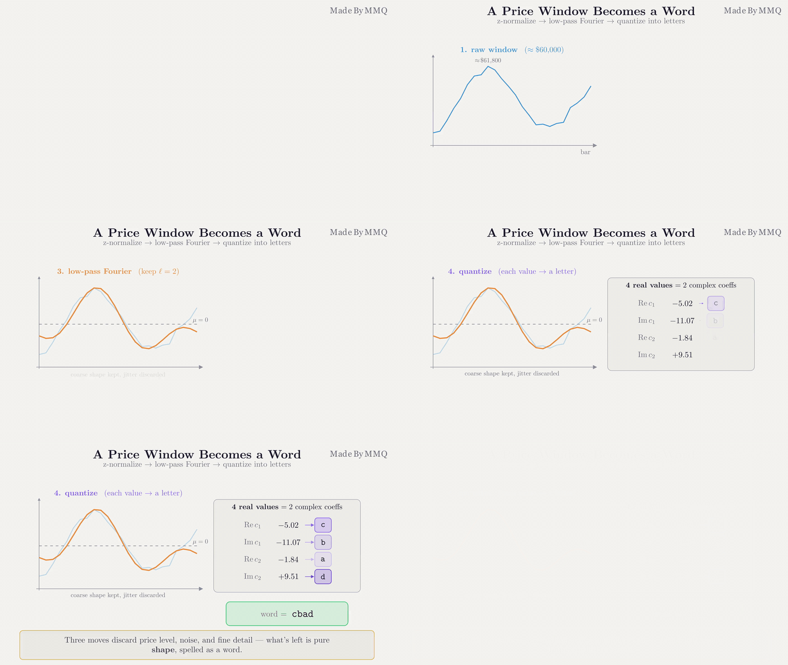
Fig. 1. A single price window is z-normalized, low-pass filtered, and quantized into a short word of letters
Symbolic Fourier Approximation (SFA)
Symbolic Fourier Approximation is the engine that turns one window into one word. It has two parts that must be built in order. First, a Fourier front end that produces the low-frequency coefficients of a window. Second, a data-driven binning scheme, Multiple Coefficient Binning (MCB), that learns how to turn those coefficients into letters. We build the Fourier part first because everything downstream depends on it.
The Fourier front end
The Discrete Fourier Transform decomposes a window into a sum of sine and cosine waves of increasing frequency. The first coefficient (the DC term) is just the window's average; the next few describe its slow, sweeping structure; the later ones describe progressively finer wiggles. For our purposes the later coefficients are noise, so we never compute more than we need. The CDFT class wraps ALGLIB's real FFT and returns only the first few coefficients, laid out as interleaved real and imaginary parts.
//+------------------------------------------------------------------+
//| CDFT - the real-input Fourier front end for SFA.                 |
//|                                                                  |
//|  SFA does not need a full spectrum. For a window of length w it  |
//|  keeps only the first 'l' complex Fourier coefficients, whose    |
//|  real and imaginary parts become the l real numbers that are     |
//|  later binned into letters. Low index = low frequency, so        |
//|  keeping the first few coefficients is a low-pass filter: it     |
//|  retains the coarse shape of the window and discards the         |
//|  high-frequency jitter. That built-in denoising is the whole     |
//|  reason SFA tolerates noisy price data.                          |
//|                                                                  |
//|  The transform itself is delegated to ALGLIB's FFTR1D, a real    |
//|  FFT that accepts any window length (no power-of-two rule). We   |
//|  simply read back the coefficients we want. The class exists to  |
//|  give SFA one clean call and to fix the coefficient-ordering     |
//|  convention in a single place.                                   |
//+------------------------------------------------------------------+
The actual transform is short. We copy the window into a plain array, call the FFT, and read back f[1..coeff_count], deliberately skipping f[0]. After z-normalization the DC term is zero, so carrying it would waste a letter on a constant.
//+------------------------------------------------------------------+
//| Compute the low-frequency coefficients of a real window.         |
//|                                                                  |
//|  'raw' is expected to be already z-normalized by the caller so   |
//|  that the DC term is ~0 and every window is compared on shape,   |
//|  not on price level. We still start reading at f[1] regardless,  |
//|  so a non-normalized window simply loses its mean here.          |
//+------------------------------------------------------------------+
bool CDFT::LowCoefficients(const double &raw[],int len,
                           int coeff_count,double &out[])
  {
   if(len<2 || coeff_count<1)
      return false;
   if(coeff_count>MaxCoefficients(len))
      return false;

//--- ALGLIB needs a plain double[] of exactly 'len' samples.
   double sample[];
   ArrayResize(sample,len);
   for(int i=0;i<len;i++)
      sample[i]=raw[i];

   complex spectrum[];
   CAlglib::FFTR1D(sample,len,spectrum);
   if(ArraySize(spectrum)<coeff_count+1)   // need f[1..coeff_count]
      return false;

//--- flatten f[1..coeff_count] into interleaved real/imag pairs.
   ArrayResize(out,coeff_count*DFT_REALS_PER_COEFF);
   for(int k=0;k<coeff_count;k++)
     {
      complex c=spectrum[k+1];             // skip f[0] (DC)
      out[DFT_REALS_PER_COEFF*k]  =c.real;
      out[DFT_REALS_PER_COEFF*k+1]=c.imag;
     }
   return true;
  }
Because each coefficient is a complex number, keeping l coefficients gives us 2l real values (a real and an imaginary part each). Those 2l numbers are the raw material for the word: each one will become a letter. Note that ALGLIB's real FFT accepts any window length, so we are not forced into power-of-two windows, and the window length stays a free parameter we can tune later. The MaxCoefficients helper enforces the ceiling: a length-w window can supply at most floor(w/2) non-DC coefficients, so a request for more than that is rejected before we ever call the FFT.
The shared foundation: z-normalization
Before any window is transformed, it is z-normalized, and this step is important enough that both the binning stage and the encoding stage call one shared implementation, so they can never drift apart. Z-normalization subtracts the mean and divides by the standard deviation, which is what strips out the price level and leaves pure shape. It also gives us a natural place to reject flat windows: if the standard deviation is essentially zero, dividing by it is meaningless, so we return false and let the caller skip that window entirely. Note that we use the population variance (dividing by len, not len-1), which is the convention the whole pipeline assumes.
//+------------------------------------------------------------------+
//| Free helper: z-normalize src[0..len-1] into dst[].               |
//|  Returns false on a flat window (stdev below SFA_FLAT_EPS),      |
//|  leaving dst[] resized but unfilled. Defined at file scope so    |
//|  both CMCB and CSFA share one z-norm and cannot drift apart.     |
//+------------------------------------------------------------------+
bool ZNorm(const double &src[],int len,double &dst[])
  {
   if(len<=0)
      return false;
   double mean=0.0;
   for(int i=0;i<len;i++)
      mean+=src[i];
   mean/=len;

   double var=0.0;
   for(int i=0;i<len;i++)
     {
      double d=src[i]-mean;
      var+=d*d;
     }
   var/=len;                               // population variance
   double sd=MathSqrt(var);
   if(sd<SFA_FLAT_EPS)
      return false;

   ArrayResize(dst,len);
   for(int i=0;i<len;i++)
      dst[i]=(src[i]-mean)/sd;
   return true;
  }
Learning the letters: Multiple Coefficient Binning
Now the interesting part, and the piece that distinguishes SFA from the older SAX method. To turn a coefficient value into a letter, we need breakpoints: cut points that divide the number line into bands, one band per letter. SAX assumes every value is drawn from a standard normal distribution and places its breakpoints at fixed Gaussian quantiles. That assumption is convenient but wrong for Fourier coefficients, whose spread varies dramatically from one coefficient to the next.
MCB refuses that assumption. It learns the breakpoints from training data, and it learns a separate set of breakpoints for each of the 2l coefficient slots. For a given slot, it collects that slot's value across every training window, sorts them, and places the breakpoints at equal-count (equi-depth) quantiles, so that each letter is used about equally often. The class header lays out the reasoning:
//+------------------------------------------------------------------+
//| CMCB - Multiple Coefficient Binning.                             |
//|                                                                  |
//|  This is the one piece that separates SFA from the older SAX.    |
//|  SAX assumes every value is drawn from a standard normal and     |
//|  cuts the alphabet at fixed Gaussian quantiles. SFA makes no     |
//|  such assumption: it LEARNS the cut points from data, and it     |
//|  learns a SEPARATE set of cuts for each Fourier coefficient,     |
//|  because a low-frequency coefficient and a high-frequency one    |
//|  have very different spreads.                                    |
//|                                                                  |
//|  Fit() takes a pile of training windows, transforms each to its  |
//|  first 'l' coefficients (l = word length x nothing extra; each   |
//|  coefficient is one real and one imaginary value, so there are   |
//|  2l real series to bin). For every one of those 2l positions it  |
//|  collects the value across all windows, sorts them, and places   |
//|  alpha-1 breakpoints at equal-count (equi-depth) quantiles so    |
//|  that each of the 'alpha' letters is used about equally often.   |
//|                                                                  |
//|  The result is a breakpoint table m_break[pos][b], pos in        |
//|  0..2l-1, b in 0..alpha-2. Symbolizing a value is then a simple  |
//|  lookup: count how many breakpoints it exceeds.                  |
//+------------------------------------------------------------------+
The fitting routine is worth reading in full, because its structure is not obvious. It runs in two passes. The first pass transforms every training window once and stores all of its coefficient slots into a flat matrix, one row per usable window. We do this rather than transforming twice because the FFT is the expensive step, and we need every window's contribution to every slot before we can bin any slot. Along the way, windows that fail z-normalization (the flat ones) or the DFT are silently skipped, and a running usable count tracks how many genuinely made it in. The second pass then bins each of the 2l slots independently: it gathers that slot's value across every usable window, sorts them, and drops the breakpoints at equal-count quantiles.
//+------------------------------------------------------------------+
//| Learn equi-depth breakpoints for every coefficient slot.         |
//|                                                                  |
//|  For each of the 2*word_len real/imag slots we gather that       |
//|  slot's value from every non-flat training window, sort the      |
//|  collection, and cut it into 'alphabet' equal-count bins. The    |
//|  b-th breakpoint sits at quantile (b+1)/alphabet, so bin 0 holds |
//|  the lowest values, bin alphabet-1 the highest, each with about  |
//|  the same number of training points.                             |
//+------------------------------------------------------------------+
bool CMCB::Fit(const double &windows[],int count,int win_len,
               int word_len,int alphabet)
  {
   m_fitted=false;
   if(count<=0 || win_len<2)
      return false;
   if(word_len<SFA_MIN_WORDLEN || word_len>SFA_MAX_WORDLEN)
      return false;
   if(alphabet<SFA_MIN_ALPHABET || alphabet>SFA_MAX_ALPHABET)
      return false;
   if(word_len>CDFT::MaxCoefficients(win_len))
      return false;

   m_dims=word_len*DFT_REALS_PER_COEFF;
   m_alphabet=alphabet;

//--- transform every training window and stack the coefficient
//--- slots column by column. 'col' holds slot 'pos' across windows.
   double coeffs[];       // reused per window: 2*word_len reals
   double norm[];         // reused per window: z-normalized samples
   double raw[];          // reused per window: raw samples
   ArrayResize(raw,win_len);

   double collected[];    // all values of the current slot, all windows
   ArrayResize(m_break,m_dims*(alphabet-1));

   int usable=0;          // count of non-flat windows actually gathered

//--- first pass builds a compact per-slot matrix. To avoid a second
//--- transform pass we transform once and store all slots, then bin
//--- slot by slot.
   double all[];          // usable*m_dims coefficients, row = window
   ArrayResize(all,count*m_dims);

   for(int wi=0;wi<count;wi++)
     {
      for(int i=0;i<win_len;i++)
         raw[i]=windows[wi*win_len+i];

      if(!ZNorm(raw,win_len,norm))
         continue;        // skip flat window

      if(!CDFT::LowCoefficients(norm,win_len,word_len,coeffs))
         continue;

      for(int p=0;p<m_dims;p++)
         all[usable*m_dims+p]=coeffs[p];
      usable++;
     }

   if(usable<=0)
      return false;

//--- bin each slot independently.
   ArrayResize(collected,usable);
   for(int p=0;p<m_dims;p++)
     {
      for(int wi=0;wi<usable;wi++)
         collected[wi]=all[wi*m_dims+p];
      ArraySort(collected);

      for(int b=0;b<alphabet-1;b++)
        {
         double q=(double)(b+1)/(double)alphabet;
         m_break[p*(alphabet-1)+b]=Quantile(collected,usable,q);
        }
     }

   m_fitted=true;
   return true;
  }
The breakpoint for band b sits at quantile (b+1)/alpha, which is what makes the bins equal-count. The quantile itself is a linearly interpolated position into the sorted array, so a breakpoint can land between two observed values rather than being pinned to one of them:
//+------------------------------------------------------------------+
//| Linear-interpolated quantile of an ascending sorted array.       |
//+------------------------------------------------------------------+
double CMCB::Quantile(double &sorted[],int n,double q) const
  {
   if(n<=0)
      return 0.0;
   if(n==1)
      return sorted[0];
   double pos=q*(n-1);
   int lo=(int)MathFloor(pos);
   int hi=lo+1;
   if(hi>=n)
      return sorted[n-1];
   double frac=pos-lo;
   return sorted[lo]+frac*(sorted[hi]-sorted[lo]);
  }
Once the table is learned, turning a coefficient value into a letter is a lookup: count how many breakpoints the value exceeds. Since the breakpoints ascend, we can stop as soon as the value falls below one of them.
//+------------------------------------------------------------------+
//| Symbol code for a value at coefficient slot 'pos'.               |
//|  Counts how many of that slot's ascending breakpoints the value  |
//|  is at or above; the count is the letter 0..alphabet-1.          |
//+------------------------------------------------------------------+
int CMCB::SymbolOf(double value,int pos) const
  {
   if(!m_fitted || pos<0 || pos>=m_dims)
      return 0;
   int nb=m_alphabet-1;
   int code=0;
   for(int b=0;b<nb;b++)
     {
      if(value>=m_break[pos*nb+b])
         code++;
      else
         break;                            // breakpoints ascend: stop early
     }
   return code;
  }
Assembling the word
The CSFA class ties the two pieces together. It is configured once with a word length and alphabet size, learns the MCB breakpoints from training windows via Fit, and thereafter encodes any window into a word. The encode routine is the three-step pipeline in code: z-normalize, take the low coefficients, and map each to a letter.
//+------------------------------------------------------------------+
//| Encode one raw window into a word of integer letters.            |
//+------------------------------------------------------------------+
ENUM_SFA_STATUS CSFA::Encode(const double &raw[],int len,int &word[]) const
  {
   if(!m_ready)
      return SFA_BAD_PARAMS;
   if(!m_mcb.IsFitted())
      return SFA_NOT_FITTED;
   if(len<2 || m_word_len>CDFT::MaxCoefficients(len))
      return SFA_BAD_PARAMS;

   double norm[];
   if(!ZNorm(raw,len,norm))
      return SFA_FLAT_WINDOW;

   double coeffs[];
   if(!CDFT::LowCoefficients(norm,len,m_word_len,coeffs))
      return SFA_BAD_PARAMS;

   int nsym=SymbolCount();
   ArrayResize(word,nsym);
   for(int p=0;p<nsym;p++)
      word[p]=m_mcb.SymbolOf(coeffs[p],p);
   return SFA_OK;
  }
The word comes out as integer letter codes; a companion WordToString renders them as a readable lowercase string such as "cbad". That readability is not a convenience, it is a feature we will exploit later when we print the vocabulary of a market regime. With SFA in hand, we can now turn a whole series into a bag of these words.
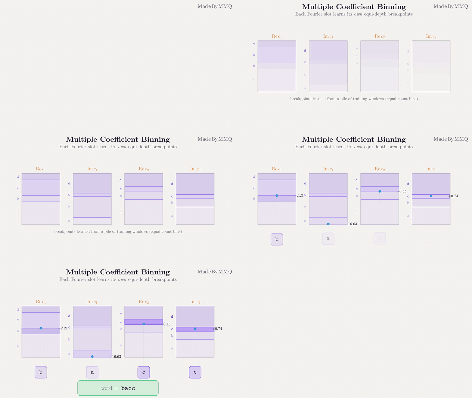
Fig. 2. SFA in full: the DFT keeps the low coefficients, and per-slot MCB breakpoints map each to a letter
From Words to a Bag: The BOSS Transform
SFA gives us one word per window. BOSS turns a whole series into a bag of words by sliding the SFA window along the series one bar at a time, encoding each position, and counting how often each word appears. The bag, a word-frequency histogram, is the fingerprint of the series. This is where the "bag-of-words" name comes from: just as a document can be summarized by how often each term appears in it, a stretch of market is summarized by how often each price-shape word appears in it.
The bag itself: a sparse histogram
Before we can fill a bag we need something to hold it. The space of possible words is large (with an alphabet of four and eight letters per word there are 4^8 possibilities), but any real series touches only a tiny fraction of them, so a dense array over the whole vocabulary would be almost entirely zeros. The CBossHistogram class stores the bag sparsely instead, as two parallel arrays: the distinct words seen, and the count of each. Adding a word is a linear search for it, incrementing if found and appending if not:
//+------------------------------------------------------------------+
//| Add one occurrence of a word.                                    |
//+------------------------------------------------------------------+
void CBossHistogram::Add(const string w)
  {
   int idx=IndexOf(w);
   if(idx>=0)
     {
      m_count[idx]++;
      return;
     }
   ArrayResize(m_word,m_size+1);
   ArrayResize(m_count,m_size+1);
   m_word[m_size]=w;
   m_count[m_size]=1;
   m_size++;
  }
The linear search sounds slow, but the vocabularies here are small (tens of distinct words per bag, not thousands), so it is perfectly adequate and keeps the structure simple. The distance function we build shortly will need to look up how often a specific word occurs, which is the same search returning the stored count or zero:
//+------------------------------------------------------------------+
//| Count of a specific word (0 if absent).                          |
//+------------------------------------------------------------------+
int CBossHistogram::CountOf(const string w) const
  {
   int idx=IndexOf(w);
   return (idx>=0)?m_count[idx]:0;
  }
Two details make filling this bag more than a naive count. The first is numerosity reduction. As the window slides one bar at a time across a quiet stretch, it often produces the same word again and again. If we counted every repeat, a long sleepy range would drown the bag in one word and swamp the genuine variety elsewhere. So a run of identical consecutive words is counted only once. The bag then measures how many distinct pattern occurrences a series contains, not how long each one lingered. The second detail is that flat windows, where SFA cannot z-normalize, simply contribute no word and break the run. Both live in the transform loop:
//+------------------------------------------------------------------+
//| Slide the window and build the numerosity-reduced word bag.      |
//+------------------------------------------------------------------+
int CBossTransform::Transform(const double &series[],int len,
                              CBossHistogram &hist) const
  {
   hist.Clear();
   if(!IsReady() || len<m_window || m_window<2)
      return -1;

   double win[];
   ArrayResize(win,m_window);
   int    word[];
   string prev="";                        // last word added (for run collapse)
   int    added=0;
   int    last=len-m_window;

   for(int start=0;start<=last;start++)
     {
      for(int i=0;i<m_window;i++)
         win[i]=series[start+i];

      if(m_sfa.Encode(win,m_window,word)!=SFA_OK)
        {
         prev="";                          // break the run across a flat gap
         continue;
        }

      string w=m_sfa.WordToString(word);
      if(w==prev)
         continue;                         // numerosity reduction: skip repeat

      hist.Add(w);
      prev=w;
      added++;
     }
   return added;
  }
Comparing two bags: the BOSS distance
To classify a new series we need a distance between its bag and each training bag, and here BOSS makes a deliberate and unusual choice: its distance is not symmetric. Given a query bag q and a sample bag s, the BOSS distance is an ordinary squared-Euclidean distance over word counts, but summed only over the words that actually occur in the query:
D(q, s) = sum over words w with q[w] > 0 of ( q[w] - s[w] )^2
Words that appear only in the sample are ignored entirely. The intuition is that a match should be judged by whether the sample reproduces the patterns the query contains, and not penalized for extra patterns the query never had. This asymmetry is one of the reasons BOSS outperforms a plain Euclidean comparison on noisy series, so we implement it exactly rather than quietly symmetrizing it. In code it is a single loop over the query's words:
//+------------------------------------------------------------------+
//| Non-symmetric BOSS distance from query q to sample s.            |
//|  Sum of squared count differences over words present in q only.  |
//+------------------------------------------------------------------+
double CBossClassifier::BossDistance(const CBossHistogram &q,const CBossHistogram &s)
  {
   double d=0.0;
   int n=q.Size();
   for(int i=0;i<n;i++)
     {
      string w=q.WordAt(i);
      double diff=(double)q.CountAt(i)-(double)s.CountOf(w);
      d+=diff*diff;
     }
   return d;
  }
Classification is then nearest-neighbor. The CBossClassifier class stores one labeled bag per training example. Adding an example is just transforming its series into a bag and appending that bag with its label; the transform happens once, at add time, so classification later is cheap:
//+------------------------------------------------------------------+
//| Transform one labelled series and store it as a training bag.    |
//+------------------------------------------------------------------+
bool CBossClassifier::AddExample(const double &series[],int len,const string label)
  {
   if(!IsReady() || len<BOSS_MIN_SERIES)
      return false;

   CBossHistogram h;
   if(m_transform.Transform(series,len,h)<0)
      return false;

   ArrayResize(m_train,m_ntrain+1);
   ArrayResize(m_label,m_ntrain+1);
   h.CopyTo(m_train[m_ntrain]);
   m_label[m_ntrain]=label;
   m_ntrain++;
   return true;
  }
The nearest-neighbor search lives in a small helper, ClassifyBag, which scans the stored bags and returns the label of the closest under the BOSS distance. It takes a skip index, which is unused for ordinary classification (we pass -1) but becomes essential for the leave-one-out scoring the ensemble needs, where a bag must be classified against every bag except itself:
//+------------------------------------------------------------------+
//| 1-NN over the stored bags, optionally skipping index 'skip'.     |
//+------------------------------------------------------------------+
string CBossClassifier::ClassifyBag(const CBossHistogram &q,int skip) const
  {
   double best=DBL_MAX;
   string lab="";
   for(int i=0;i<m_ntrain;i++)
     {
      if(i==skip)
         continue;
      double d=BossDistance(q,m_train[i]);
The public Classify method wraps it: it transforms the incoming series into a query bag, delegates to ClassifyBag for the winning label, and then does one cheap re-scan to recover the winning distance for the caller. It works, but as we are about to see, a single such classifier is not yet the method that competes.
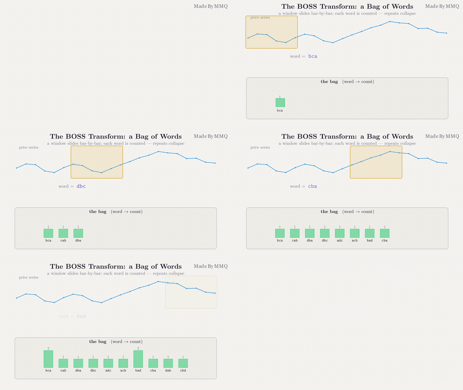
Fig. 3. The sliding window builds a bag of words; numerosity reduction collapses runs of repeats
Why One BOSS Is Not Enough: The Ensemble
A single BOSS classifier commits to one sliding-window length. That is a problem, because the right window length is data-dependent and not known in advance: a short window captures fast, local structure and misses slow sweeps, while a long window does the reverse. Pick wrong and the classifier is blind to exactly the structure that distinguishes your classes. In our own testing, a single BOSS on real data performed poorly precisely for this reason, and it is a well-documented weakness of the method.
The fix, and the version of BOSS that is actually competitive, is the ensemble. Rather than gambling on one window size, it trains one BOSS member at each of several window sizes, scores each member, keeps only the good ones, and lets them vote. The scoring uses leave-one-out training accuracy: each training bag is classified against all the others, and the fraction correctly labeled is the member's score. Members whose score comes within a fixed fraction (the literature uses 92%) of the best member are retained; the rest are discarded. A query is then classified by majority vote among the survivors.
//+------------------------------------------------------------------+
//| Leave-one-out training accuracy.                                 |
//|  Each stored bag is classified against all the others; the       |
//|  fraction whose predicted label matches the stored one is the    |
//|  member's LOO accuracy. The ensemble keeps only members whose    |
//|  LOO accuracy is close to the best (Schaefer's 92% rule).        |
//+------------------------------------------------------------------+
double CBossClassifier::LooAccuracy(void) const
  {
   if(m_ntrain<2)
      return 0.0;
   int correct=0;
   for(int i=0;i<m_ntrain;i++)
     {
      string pred=ClassifyBag(m_train[i],i);   // skip self
      if(pred==m_label[i])
         correct++;
     }
   return (double)correct/(double)m_ntrain;
  }
The CBossEnsemble class owns the whole procedure. Because different members use different window sizes, and each window size needs its own MCB breakpoints and its own labeled bags, the ensemble is handed the raw labeled segments and builds each member's pool and bags internally. That per-member setup is done by FitMember, and it is worth showing because it is the piece that makes the different window sizes work. For a given window length it harvests every sliding window across every training segment into one big MCB pool, fits a fresh CBossClassifier on that pool, and then adds each whole training segment back as one labeled bag:
//+------------------------------------------------------------------+
//| Build one member at a given window size from the stored segments.|
//|  Harvests every sliding window inside every training segment for |
//|  the MCB pool, then adds each segment as one labelled bag.       |
//+------------------------------------------------------------------+
bool CBossEnsemble::FitMember(int win_len,CBossClassifier &clf) const
  {
   if(win_len<2 || win_len>m_seglen)
      return false;

//--- MCB pool: all sliding windows across all training segments.
   int perSeg=m_seglen-win_len+1;
   int poolN=m_nseg*perSeg;
   if(poolN<=0)
      return false;
   double pool[];
   ArrayResize(pool,poolN*win_len);
   int pk=0;
   for(int s=0;s<m_nseg;s++)
      for(int start=0;start<=m_seglen-win_len;start++)
        {
         for(int j=0;j<win_len;j++)
            pool[pk*win_len+j]=m_seg[s*m_seglen+start+j];
         pk++;
        }

   if(!clf.Build(m_word_len,m_alphabet,pool,poolN,win_len))
      return false;

//--- add each training segment as one labelled bag.
   double ex[];
   ArrayResize(ex,m_seglen);
   for(int s=0;s<m_nseg;s++)
     {
      for(int j=0;j<m_seglen;j++)
         ex[j]=m_seg[s*m_seglen+j];
      clf.AddExample(ex,m_seglen,ClassName(m_lab[s]));
     }
   return true;
  }
With FitMember in hand, the training loop fits a candidate at every requested window size, records its LOO accuracy, tracks the best, and then keeps the members that clear the 92% cutoff:
//--- fit a candidate member at each window size and score it.
   CBossClassifier cand[];
   int    cwin[];
   double cacc[];
   ArrayResize(cand,nwin);
   ArrayResize(cwin,nwin);
   ArrayResize(cacc,nwin);
   int ncand=0;
   double best=0.0;

   for(int w=0;w<nwin && ncand<BOSS_MAX_MEMBERS;w++)
     {
      int win_len=wins[w];
      if(word_len>win_len/2)               // need >= word_len non-DC coeffs
         continue;
      if(!FitMember(win_len,cand[ncand]))
         continue;
      double acc=cand[ncand].LooAccuracy();
      cwin[ncand]=win_len;
      cacc[ncand]=acc;
      if(acc>best)
         best=acc;
      ncand++;
     }
   if(ncand<=0)
      return false;

//--- keep members within 92% of the best LOO accuracy.
   double cut=best*BOSS_ENSEMBLE_KEEP;
   ArrayResize(m_member,ncand);
   ArrayResize(m_win,ncand);
   ArrayResize(m_acc,ncand);
   for(int i=0;i<ncand;i++)
      if(cacc[i]>=cut)
        {
         m_win[m_count]=cwin[i];
         m_acc[m_count]=cacc[i];
         //--- rebuild the kept member into the persistent slot.
         FitMember(cwin[i],m_member[m_count]);
         m_count++;
        }
   return (m_count>0);
  }
One subtlety in that retention loop: a kept member is rebuilt into its persistent slot with a fresh FitMember call, rather than copied from the candidate array. This is deliberate, and it sidesteps the awkwardness of deep-copying classifier objects that themselves contain dynamic arrays of histograms; rebuilding is a few milliseconds and keeps the ownership clean.
Classification is the vote. Each kept member classifies the query independently, the labels are tallied, and the label with the most votes wins:
//+------------------------------------------------------------------+
//| Classify a query segment by majority vote of the kept members.   |
//|  Ties are broken by the earliest-listed label reaching the top   |
//|  count, which is deterministic given the member order.           |
//+------------------------------------------------------------------+
string CBossEnsemble::Classify(const double &series[],int len) const
  {
   if(m_count<=0)
      return "";

//--- tally votes as (label,count) pairs.
   string vlab[];
   int vcnt[];
   int nv=0;
   ArrayResize(vlab,m_count);
   ArrayResize(vcnt,m_count);

   for(int i=0;i<m_count;i++)
     {
      double bd;
      string lab=m_member[i].Classify(series,len,bd);
      if(lab=="")
         continue;
      int found=-1;
      for(int v=0;v<nv;v++)
         if(vlab[v]==lab)
           {
            found=v;
            break;
           }
      if(found<0)
        {
         vlab[nv]=lab;
         vcnt[nv]=1;
         nv++;
        }
      else
         vcnt[found]++;
     }

   string best="";
   int bestc=-1;
   for(int v=0;v<nv;v++)
      if(vcnt[v]>bestc)
        {
         bestc=vcnt[v];
         best=vlab[v];
        }
   return best;
  }
As we will see in the benchmark, this single change, from one window size to a voting ensemble of them, is the difference between BOSS losing badly and BOSS winning. It is not a minor tuning detail; it is the method.
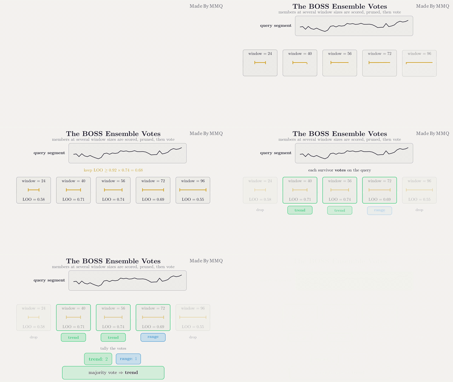
Fig. 4. Several BOSS members at different window sizes classify the query, and the majority vote wins
Labeling Market Regimes Without Hand-Labeling
BOSS is a supervised classifier: it learns from labeled examples. To teach it market regimes we need labeled segments of price, and hand-labeling thousands of them is neither practical nor reproducible. Instead we derive the labels mechanically, from two classic statistics of a segment's log returns. This gives us a transparent, deterministic ground truth that BOSS must then learn to reproduce from window shape alone.
The two statistics are:
- Lag-1 autocorrelation of returns. When consecutive returns are positively correlated, moves tend to continue, which is the signature of a trend. When it is near zero or negative, moves tend to reverse, which is the signature of a range.
- Return volatility (standard deviation), judged against a rolling reference so that "high" is relative to the instrument rather than an absolute number. An unusually wild segment is volatile.
Both statistics operate on log returns, not raw prices, so the first step is always to convert a price window into its returns. We guard against non-positive prices (which would break the logarithm) and simply skip those pairs:
//+------------------------------------------------------------------+
//| Fill ret[0..len-2] with log returns of price[0..len-1].          |
//| Returns the number of returns produced.                          |
//+------------------------------------------------------------------+
double CRegimeLabeler::LogReturns(const double &price[],int len,double &ret[]) const
  {
   int k=0;
   ArrayResize(ret,MathMax(0,len-1));
   for(int i=1;i<len;i++)
     {
      if(price[i-1]>0.0 && price[i]>0.0)
         ret[k++]=MathLog(price[i]/price[i-1]);
     }
   ArrayResize(ret,k);
   return k;
  }
The lag-1 autocorrelation is the ratio of the sum of products of consecutive centered returns to the sum of squared centered returns. A positive value means an up move tends to be followed by another up move (persistence, a trend); a value near or below zero means moves tend to reverse (a range):
//+------------------------------------------------------------------+
//| Lag-1 autocorrelation of a return series.                        |
//|  corr = sum((r[i]-mean)(r[i-1]-mean)) / sum((r[i]-mean)^2).      |
//+------------------------------------------------------------------+
double CRegimeLabeler::Autocorr1(const double &ret[],int n) const
  {
   if(n<3)
      return 0.0;
   double mean=0.0;
   for(int i=0;i<n;i++)
      mean+=ret[i];
   mean/=n;

   double num=0.0, den=0.0;
   for(int i=0;i<n;i++)
     {
      double d=ret[i]-mean;
      den+=d*d;
      if(i>0)
         num+=d*(ret[i-1]-mean);
     }
   if(den<=0.0)
      return 0.0;
   return num/den;
  }
Volatility is the population standard deviation of the same returns, and a companion WindowVolatility (not shown) simply chains LogReturns into StdDev so a price window can be measured in one call. This is what the benchmark uses to build the rolling reference against which "high" volatility is judged:
//+------------------------------------------------------------------+
//| Standard deviation of a return series (population).              |
//+------------------------------------------------------------------+
double CRegimeLabeler::StdDev(const double &ret[],int n) const
  {
   if(n<=0)
      return 0.0;
   double mean=0.0;
   for(int i=0;i<n;i++)
      mean+=ret[i];
   mean/=n;
   double var=0.0;
   for(int i=0;i<n;i++)
     {
      double d=ret[i]-mean;
      var+=d*d;
     }
   var/=n;
   return MathSqrt(var);
  }
The CRegimeLabeler class applies these in a fixed hierarchy: volatility dominates, so an unusually wild segment is labeled volatile whatever its autocorrelation says; among calmer segments, strong positive autocorrelation marks a trend; everything else is a range. The decision is deliberately simple and readable, because it is the benchmark's source of truth, not the thing under test:
//+------------------------------------------------------------------+
//| Label one price window as trend / range / volatile.              |
//+------------------------------------------------------------------+
ENUM_REGIME CRegimeLabeler::Label(const double &price[],int len) const
  {
   double ret[];
   int n=(int)LogReturns(price,len,ret);
   if(n<3)
      return REGIME_UNDEFINED;

   double vol=StdDev(ret,n);
   double acf=Autocorr1(ret,n);

//--- volatility first: an unusually wild window is VOLATILE whatever
//--- its autocorrelation says.
   double vol_ref=(m_ref_vol>0.0)?m_ref_vol:vol;
   if(vol>m_vol_hi_mult*vol_ref)
      return REGIME_VOLATILE;

//--- among calmer windows, strong persistence marks a trend.
   if(acf>m_acf_trend)
      return REGIME_TREND;

   return REGIME_RANGE;
  }
The two thresholds, the trend autocorrelation cutoff and the volatility multiplier, are inputs. They matter more than they might appear: set them too strict and almost every segment falls through to "range", producing a degenerate label distribution that no classifier can learn from. On BTCUSD H1 we found that loosening them to a trend cutoff of 0.05 and a volatility multiplier of 1.3 gives a workably balanced mix of the three classes, which is what the benchmark below uses.
Putting It to the Test: BOSS vs DTW
Now the empirical part. We benchmark BOSS against Dynamic Time Warping, the elastic-distance classic, on exactly the same task: classify a segment of BTCUSD H1 into trend, range, or volatile, using the same auto-generated labels and the same 1-nearest-neighbor protocol. Before we do that on messy real bars, though, it is worth confirming the classifier behaves on controlled shapes where we know the right answer.
A controlled sanity check first
BOSSSelfTest.mq5 builds three synthetic series, a trending drift, a clean oscillation, and a volatile random walk, and asks the classifier three questions in turn. It is a behavioral test on shapes with known labels, so any failure here is a bug in the engine, not an ambiguity in the market. The first question, discrimination on clean queries, is a clean pass: on well-separated shapes the classifier is perfect, scoring 90 of 90 across all three classes.
The second question is more revealing. It pushes a single ranging query through rising noise and checks whether it survives. It does not survive for long, and this is the first crack in the noise story: correct at low noise, it falls apart by the time the noise amplitude reaches half the signal, foreshadowing exactly the limitation the benchmark will confirm on real data.
| Noise amplitude | Range queries correct | Accuracy |
|---|---|---|
| 0.1 | 40/40 | 100% |
| 0.5 | 3/40 | 8% |
| 1.0 | 0/40 | 0% |
| 1.5 | 0/40 | 0% |
The third question is the interesting one: it prints the actual vocabulary of each shape, the most frequent words and how often they occur. A trending series concentrates its mass on a few words, a range is tighter still with only fourteen distinct words, and a volatile series sprawls across fifty-nine with almost no repetition, because chaos has no characteristic shape. That readable signature is a genuine analytical property, and we return to it once the benchmark is done.
| Shape | Distinct words | Top three words (with counts) |
|---|---|---|
| trend | 24 | [adbc]x12 [ddbc]x11 [bdbc]x7 |
| range | 14 | [cacb]x10 [adcb]x10 [dbcb]x9 |
| volatile | 59 | [adda]x7 [ddac]x7 [ddda]x7 |
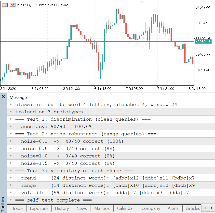
Fig. 5. The self-test terminal output: perfect discrimination on clean shapes, the per-query noise breakdown, and the vocabulary each shape produces
With the engine's behavior confirmed on shapes we control, we move to the real test. To keep the comparison against DTW fair we make three commitments up front.
- Both see shape, not price level. BOSS z-normalizes internally; we z-normalize every segment before handing it to DTW as well. Without this, DTW would match on absolute price, which is meaningless on an instrument that ranges over tens of thousands of dollars, and the comparison would be rigged against it.
- The unit of classification is a segment, not a single window. BOSS represents a series by the distribution of words its sliding window produces, so it needs a segment long enough to yield many words. We classify 120-bar segments; DTW compares the same 120-bar shapes point by point.
- We report macro accuracy, not just raw accuracy. The regime mix is imbalanced (range dominates), so a classifier that always guesses "range" can post a high raw score while being useless. Macro accuracy, the mean of the per-class recalls, exposes that, so it is the number that matters.
The benchmark cuts the history into non-overlapping segments, labels each, splits them into a training half and a test half, trains single-BOSS, the BOSS ensemble, and uses the training half as DTW's prototypes. It then classifies every test segment with all three and reports accuracy, macro accuracy, and wall-clock time per query. Here is the result on clean queries.
| Classifier | Raw accuracy | Macro accuracy | Time per query |
|---|---|---|---|
| Baseline (always "range") | 71.7% | - | - |
| Single BOSS | 49.1% | 25.3% | ~9 ms |
| BOSS ensemble | 57.2% | 62.5% | ~35 ms |
| DTW | 50.9% | 44.8% | ~735 ms |
Two things jump out. First, the ensemble is the story: single BOSS scores a dismal 25.3% macro, barely better than picking one class, while the ensemble lifts that to 62.5%. This is the "one BOSS is not enough" claim made concrete, the exact jump the previous section promised. Second, on macro accuracy the ensemble beats DTW decisively, 62.5% against 44.8%, and it does so roughly twenty times faster: about 35 milliseconds per query against DTW's 735 milliseconds, because DTW pays an O(n^2) alignment cost against every prototype while BOSS does histogram lookups. On clean data, the dictionary approach wins on both accuracy and speed.
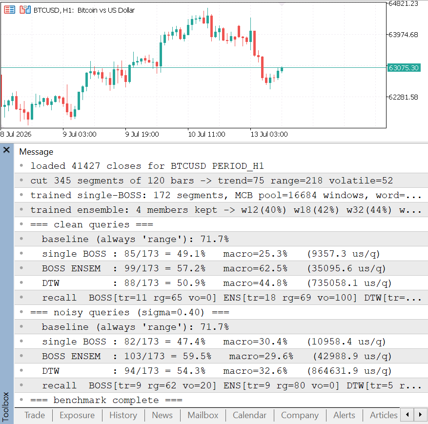
Fig. 6. The benchmark output: single BOSS, the ensemble, and DTW on clean and noisy queries
The honest limitation: noise
The introduction promised we would test the noise claim rather than assume it, and this is where we make good on that. The low-pass Fourier filter is a genuine reason to expect noise-robustness, and at the word level it delivers. But at the segment-classification level the data does not fully support the claim, and we will not hide it. When we inject noise into the test queries and re-run, the picture changes:
| Classifier (noisy queries) | Raw accuracy | Macro accuracy |
|---|---|---|
| Single BOSS | 47.4% | 30.4% |
| BOSS ensemble | 59.5% | 29.6% |
| DTW | 54.3% | 32.6% |
Under heavy noise injection the ensemble's macro accuracy collapses from 62.5% to 29.6%. DTW, at 32.6%, edges ahead. So the noise-robustness advantage that holds at the window level, the low-pass filter really does denoise individual words, does not survive at the segment-classification level once the whole bag is corrupted. The clean-data win is real; the noise-robustness claim is not, at least not for this task and this noise model. It is worth being clear about why this is a limitation and not a contradiction: the test set here is small (about 170 queries, with only a handful of volatile examples), so these noisy figures carry real variance, and the noise we inject is aggressive. But the direction is consistent enough to summarize BOSS's empirical scorecard as follows: more accurate than DTW on clean data, far faster, and interpretable. It is not, however, more noise-robust at the segment level.
The per-class recalls make the collapse concrete, and they are more revealing than the macro number alone. On clean queries the ensemble's strong macro score is carried almost entirely by the volatile class, which it recovers perfectly (100% recall), while its trend recall is weak (18%); range sits in between. Under noise, the picture inverts: volatile recall falls from 100% all the way to 0%, and the ensemble essentially stops recognizing the one class it was best at. That single swing is what drags the macro average down, and it is a clean illustration of the mechanism: once noise corrupts the bag, the distinctive vocabulary of a volatile segment (its sprawl of rarely-repeated words) is exactly what gets washed out first.
The claim that noise-robustness lives "at the word level" is not hand-waving, and it is also what pins down the one parameter we have taken on faith so far: how many Fourier coefficients to keep. BOSSNoiseSweep.mq5 isolates that word-level behavior by running the simplest possible task, trend versus range on a classifier trained at low noise (0.07), and sweeping the retained-coefficient count against rising query noise. Chance on this two-class task is 50%:
| WordLen (coefficients / letters) | noise=0.1 | noise=0.3 | noise=0.5 | noise=1.0 | noise=1.5 |
|---|---|---|---|---|---|
| 2 (4L) | 100% | 100% | 100% | 88% | 74% |
| 3 (6L) | 100% | 69% | 52% | 58% | 64% |
| 4 (8L) | 100% | 61% | 69% | 84% | 64% |
The pattern is clean and it decides the parameter. Keeping only two coefficients (a four-letter word) holds at or near 100% until the noise is heavy, and even at the extreme it stays well above chance. Keeping more coefficients, longer words that capture finer shape detail, does the opposite: they overfit the noise and collapse toward the 50% coin-flip almost as soon as any noise appears. Fewer coefficients means a stronger low-pass filter, and a stronger low-pass filter is exactly what survives noise. This is why every classifier in this article uses WordLen=2: it is not a default, it is the measured robust operating point for this window size.
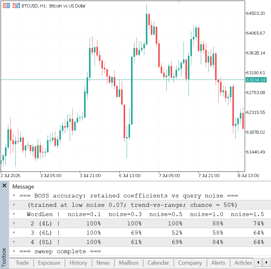
Fig. 7. The coefficient-sweep terminal output: two coefficients stay robust under noise while longer words overfit and collapse
Interpretability: reading the vocabulary
There is one thing BOSS offers that DTW structurally cannot: you can read its vocabulary. We saw this already in the self-test's vocabulary table, where each shape printed its own dialect; the same property holds on real regimes. Because each bag is literally a table of words and counts, we can print the most frequent words a regime produces and see its dialect. A ranging market produces a small, tight vocabulary dominated by a few oscillation words; a volatile market produces a sprawling vocabulary with almost no repetition, because chaos has no characteristic shape. That readable signature is a genuine analytical advantage, and it is why symbolic methods remain attractive even where a black-box model might edge them on raw accuracy.
The Regime Indicator
The payoff of all this machinery is a tool you can attach to a chart. BOSSRegime.mq5 is a self-contained indicator that trains a BOSS ensemble on recent history when it loads, then tags every bar with the regime of the segment ending at it, drawing a color-coded lane in a separate window: blue for range, green for trend, red for volatile. Any Expert Advisor can read that lane as context, gating its strategy on the current regime.
Everything happens in two places. On initialization the indicator binds its plot buffers and trains the ensemble once, refusing to run if training fails:
//+------------------------------------------------------------------+
//| Indicator init: bind buffers, train the ensemble.                |
//+------------------------------------------------------------------+
int OnInit()
  {
   SetIndexBuffer(0,RegimeBuffer,INDICATOR_DATA);
   SetIndexBuffer(1,ColorBuffer,INDICATOR_COLOR_INDEX);
   IndicatorSetString(INDICATOR_SHORTNAME,"BOSS Regime");
   IndicatorSetInteger(INDICATOR_DIGITS,0);
   PlotIndexSetDouble(0,PLOT_EMPTY_VALUE,EMPTY_VALUE);

   g_ready=TrainEnsemble();
   if(!g_ready)
      return INIT_FAILED;
   return INIT_SUCCEEDED;
  }
Then, on each calculation, it tags the new bars. It only recomputes bars that have appeared since the last call, so it stays cheap after the initial pass, and it classifies each bar by the trailing segment of closes ending at that bar:
//--- OnCalculate delivers close[] in chronological order (index 0 =
//--- oldest), which is exactly what segment slicing expects. Index i
//--- is the bar whose trailing Segment closes end at i.
   int start=(prev_calculated>0)?prev_calculated-1:Segment;
   if(start<Segment)
      start=Segment;

   ENUM_REGIME lastReg=REGIME_UNDEFINED;
   for(int i=start;i<rates_total;i++)
      lastReg=ClassifyBarSegment(close,i,i);
The classification itself reuses the trained ensemble directly: slice out the Segment closes ending at the bar, call the ensemble's Classify, and write the regime code and color index into the plot buffers. Because the ensemble was trained once at load time, tagging a bar is only a few histogram comparisons, fast enough to run live.
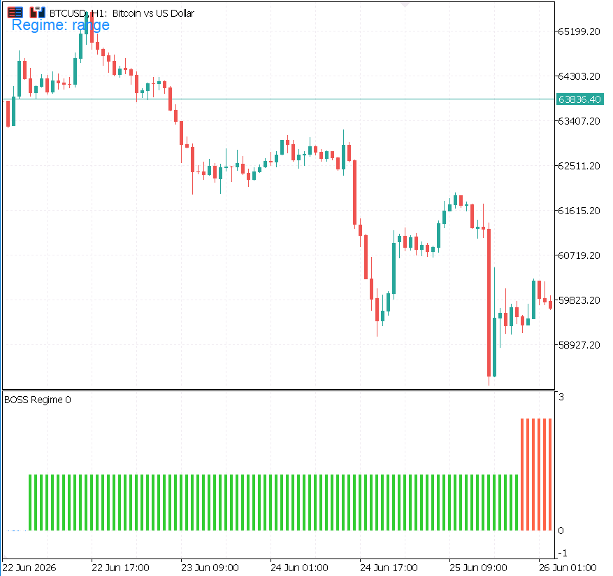
Fig. 8. The color-coded regime lane under a BTCUSD H1 chart: blue range, green trend, red volatile
Conclusion
We built the Bag-of-SFA-Symbols classifier from the ground up in pure MQL5, turning windows of price into words with Symbolic Fourier Approximation, words into bags with the BOSS transform, and bags into a competitive classifier with the ensemble, then tested the whole thing empirically against Dynamic Time Warping on real BTCUSD data.
- A complete, reusable engine. CDFT, CMCB, CSFA, CBossTransform, CBossClassifier, and CBossEnsemble form a self-contained symbolic time-series toolkit with no external dependencies beyond ALGLIB's FFT, usable for any classification task, not only regimes.
- The ensemble is the method. A single BOSS scored 25.3% macro accuracy and lost; the ensemble scored 62.5% and won. The lesson generalizes: for dictionary classifiers, voting across window sizes is not an optional refinement, it is what makes them work.
- A real win, honestly bounded. On clean data the BOSS ensemble beat DTW on balanced accuracy (62.5% against 44.8%) and ran roughly twenty times faster. Under heavy noise injection, however, DTW edged ahead, so we do not claim noise robustness at the segment level, and we showed the numbers that make that case.
- Interpretability for free. BOSS's vocabulary is readable: a regime has a dialect you can print and inspect, something no elastic-distance method offers.
There are natural next steps. A richer labeler, or forward-looking labels tied to realized behavior, would give BOSS a cleaner target to learn. WEASEL, a successor to BOSS that weights discriminative words and mixes window lengths more aggressively, is a promising direction for the noise problem. And the ensemble's members and thresholds are all tunable, so there is room to push the accuracy further.
Getting the Source Code via MQL5 Algo Forge
All source files are attached to this article below, but the full repository is also available on MQL5 Algo Forge, the community's Git-based platform for sharing and collaborating on trading projects.
| File name | Description |
|---|---|
| MQL5\Include\BOSS\FourierTransform.mqh | CDFT: real-input Fourier front end (ALGLIB FFT), returns the low coefficients for SFA |
| MQL5\Include\BOSS\SFA.mqh | CMCB (Multiple Coefficient Binning) and CSFA (Symbolic Fourier Approximation): window to word |
| MQL5\Include\BOSS\BOSS.mqh | CBossTransform, CBossClassifier, and CBossEnsemble: bag-of-words, BOSS distance, and the voting ensemble |
| MQL5\Include\BOSS\RegimeLabeler.mqh | CRegimeLabeler: rule-based trend/range/volatile labels from autocorrelation and volatility |
| MQL5\Indicators\BOSS\BOSSRegime.mq5 | Self-contained regime indicator: trains a BOSS ensemble and color-codes the regime lane |
| MQL5\Scripts\BOSS\BOSSvsDTWBenchmark.mq5 | Head-to-head benchmark of single BOSS, the ensemble, and DTW on real bars |
| MQL5\Scripts\BOSS\BOSSSelfTest.mq5 | Behavioral self-test of the classifier on synthetic shapes, with a vocabulary readout |
| MQL5\Scripts\BOSS\BOSSNoiseSweep.mq5 | Diagnostic sweep of retained-coefficient count against query noise |
Warning: All rights to these materials are reserved by MetaQuotes Ltd. Copying or reprinting of these materials in whole or in part is prohibited.
This article was written by a user of the site and reflects their personal views. MetaQuotes Ltd is not responsible for the accuracy of the information presented, nor for any consequences resulting from the use of the solutions, strategies or recommendations described.

 Building a Volume-Based Liquidity Heatmap Indicator in MQL5
 Crystal Structure Algorithm (CryStAl)
 Exporting Custom Indicator Buffers to CSV for Python Backtesting Pipelines
 Building a Divergence System (Part III): The Adaptive SuperTrend EA

- Free trading apps
- Over 8,000 signals for copying
- Economic news for exploring financial markets
You agree to website policy and terms of use