Measuring Market Efficiency with Lempel-Ziv Complexity

Contents

1. Introduction
2. What the tool does, and its one honest warning
3. Lempel-Ziv complexity: compression without a compressor
4. Turning a price window into symbols with SAX
5. Building the library
6. Comparing two windows: Normalized Compression Distance
7. Testing it to death
8. The efficiency indicator
9. Reading real markets without fooling yourself
10. Limitations and honest scope
11. Conclusion

Introduction

There is an old intuition behind data compression: a file compresses well when it is repetitive, and badly when it is random. A ZIP archive of a text full of repeated words is tiny, while an archive of random bytes is barely smaller than the original. The same idea can be pointed at a price series. If the recent bars carry a repeating structure, a good parser needs few pieces to describe them. If they are effectively noise, it needs many. That count is a direct measure of how much repeatable regularity is present.

This is attractive because most predictability measures come with knobs. An autocorrelation test needs a lag, a spectral method needs a window and a taper, a machine-learning model needs features and hyperparameters. Lempel-Ziv complexity needs none of that. You feed it a sequence of symbols and it returns an integer: the number of distinct phrases it had to invent while reading the sequence left to right. Normalize that integer and you get a number that sits near 1 for noise and near 0 for a perfectly regular series.

One honesty has to travel with that claim, because the rest of the article depends on it. The complexity formula itself takes no parameters, but it does not act on raw prices. Turning a price window into symbols requires choices: window length, alphabet size, optional aggregation, and whether to read returns or levels. The formula adds no knobs of its own, yet the measure as a whole is a small stack of deliberate choices, and each one is named where it is introduced. So the parameter-free property belongs to the LZ count, not to the pipeline around it.

The idea has a name in finance. The efficient-market hypothesis says that in a liquid market prices already reflect the available information, so returns should be close to unpredictable, close to a coin flip. Compression turns that abstract claim into something you can measure on a chart. If the moves are truly unpredictable they do not compress, and the complexity reads high. Where the complexity drops, the market is, in this narrow sense, leaving structure on the table. Whether that structure is anything you could trade is a harder question, and one this article takes seriously rather than waving away.

The catch, and the reason this article spends as much time on measurement discipline as on code, is that a raw complexity reading on real returns is easy to misread. Market returns are fat-tailed, and fat tails lower the complexity number on their own, with no predictability behind them at all. So a naive reading calls an efficient market inefficient. The library here is built to separate the two: what part of a low reading is the shape of the return distribution, and what part is genuine structure you could act on.

The work is aimed at a developer who wants a compact, well-tested complexity toolkit in pure MQL5, and who cares more about an honest answer than a flattering one. Everything is built from scratch, cross-checked against an independent Python implementation, and then run on EURUSD and gold across two timeframes.

What the tool does, and its one honest warning

The deliverable is an indicator that plots one line in a subwindow: the normalized Lempel-Ziv complexity of the trailing window of log-returns, symbolized with SAX. The line lives on a fixed scale. A value near 1.0 means the recent moves look like independent coin flips, an efficient tape with no memory. A value clearly below 1.0 means the moves carry serial structure, some repeatable pattern in how one bar follows another.

The screenshot below shows the indicator attached to a chart in its own pane, with a dotted reference line at 1.0. Above the line is noise, below it is structure.

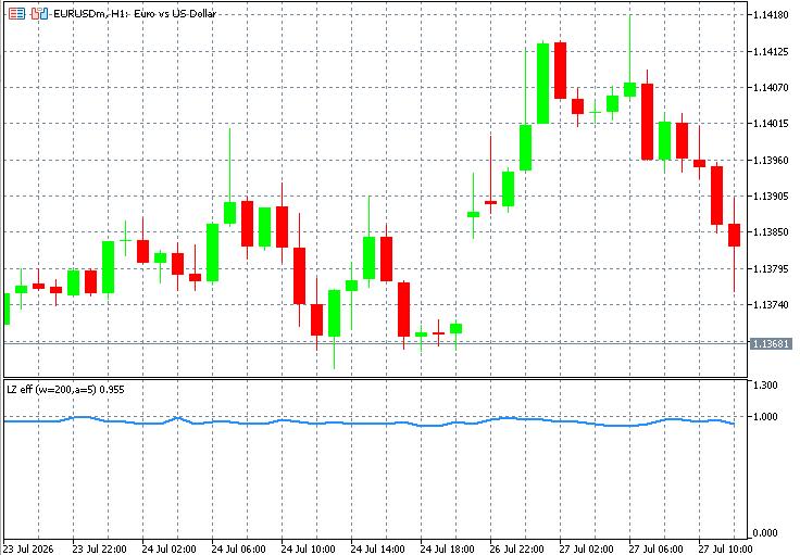
Fig. 1. The efficiency indicator in its own pane below the price chart, with the dotted reference line at 1.0 separating noise above from structure below

There is one warning that the whole second half of this article exists to justify, so it belongs up front. The efficiency line answers "how random are the moves", not "is price going up". A steady drift does not pull the line down, because the symbolizer removes the level and scale before measuring, so a trend riding on ordinary noise symbolizes as noise. This holds for a steady drift, not for every shape. If the slope keeps changing or the run is sharply one-sided, the path can remain deterministic after z-normalization. In that case, the measure should read it as structure, because it is not noise. A reading below 1.0 does not mean the market is tradable. Fat tails alone can lower the reading without any predictability. The library reports the number; interpreting it requires controls, which the market-scan section provides.

That is what this article delivers: the measure, the library that computes it, and the discipline to read it. The rest explains how.

Lempel-Ziv complexity: compression without a compressor

Lempel and Ziv defined a complexity measure in 1976 that counts the number of new phrases needed to build a sequence from left to right. Start at the beginning. Read forward until you reach a piece that cannot be copied from what you have already seen. That piece closes a phrase, the counter ticks, and you continue from there. A sequence full of repetition lets you copy long stretches, so few phrases open. A random sequence forces a new phrase every few symbols.

The picture below makes this concrete on two binary strings. The periodic string 0 1 0 1 ... is described in only three phrases: the parser learns "0", then "1", and then copies the alternating pattern to the end in a single long phrase. The random string keeps surprising the parser, so a new phrase opens again and again. Each colored block is one phrase.

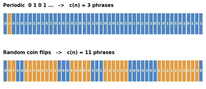
Fig. 2. The LZ76 phrase parse of a periodic string and a random one; the periodic string collapses into three phrases while the random string opens a new phrase again and again

The count itself, written c(n), depends on the length n and the alphabet size. To compare windows of different lengths on one scale, it is normalized. For a random sequence over an alphabet of size a, c(n) grows like n divided by log_a(n), so dividing by that limit gives a number that tends to 1 for noise:

C = c(n) * log_a(n) / n = c(n) * ln(n) / (n * ln a)

The division has a plain reading. A random string over five symbols cannot be compressed, so its phrase count grows as fast as the theory allows and the ratio lands near 1. A string with structure opens fewer phrases than that ceiling, so the ratio falls toward 0. Length drops out of the arithmetic, which is what lets a 200-bar window and a 300-bar window be placed on the same axis and compared directly.

The next figure shows this normalized value for four synthetic symbol strings of the same length. A constant string sits near zero, short periods stay low, and a random string sits near the dashed limit at 1.0. This is the full working range of the measure.

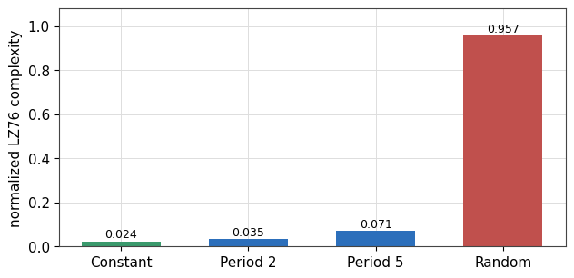
Fig. 3. Normalized LZ76 complexity for four strings of the same length, rising from a constant near zero through short periods to a random string close to one

The computation is the Kaspar and Schuster (1987) formulation, kept as a plain index walk so it stays fast and easy to mirror in another language. Here is the whole routine, byte for byte from the library.

//+------------------------------------------------------------------+
//| LZ76 complexity - Kaspar & Schuster index walk                   |
//|                                                                  |
//|  i     : start of the reconstruction window in the history       |
//|  l     : start of the phrase currently being built               |
//|  k     : length matched so far from position i                   |
//|  k_max : longest match found while sweeping i over [0, l)        |
//|  c     : phrase count (the complexity)                           |
//+------------------------------------------------------------------+
int CLZComplexity::Complexity(const uchar &symbols[], int n) const
  {
   if(n <= 0)
      return 0;
   if(n == 1)
      return 1;

   int i = 0, k = 1, l = 1;
   int k_max = 1;
   int c = 1;

   while(true)
     {
      if(symbols[i + k - 1] == symbols[l + k - 1])
        {
         k++;
         if(l + k > n)
           {
            c++;
            break;
           }
        }
      else
        {
         if(k > k_max)
            k_max = k;
         i++;
         if(i == l)
           {
            c++;
            l += k_max;
            if(l + 1 > n)
               break;
            i     = 0;
            k     = 1;
            k_max = 1;
           }
         else
            k = 1;
        }
     }
   return c;
  }

The two pointers do the work. l marks the start of the phrase being built, i sweeps every earlier start position looking for the longest match, and k measures how far that match runs. When no earlier position can reproduce the piece, k_max records the best attempt, the phrase advances by that length, and c increments. The self-reference is deliberate: a match may run forward into the current phrase, which is what lets a long periodic run collapse into a single phrase. The routine has no allocations and no recursion, so it is cheap enough to call on every bar.

Tracing the count on a short string makes the mechanic clear. Take 0001101001000101, the example from the original paper. Reading left to right, the parser opens a new phrase every time the piece ahead of it cannot be copied from the history already read, and on this string it opens six of them before it reaches the end. That is the value the routine returns, and it is one of the fixed numbers the tests below pin down, so a change to the algorithm that quietly altered it would be caught at once.

Turning a price window into symbols with SAX

Complexity is defined on symbols, not on real numbers, so a price window has to be discretized first. The naive choice is one bit per bar: up is 1, down is 0. That throws away the size of every move, which is exactly the information that separates a calm drift from a violent reversal. The library uses SAX instead, the Symbolic Aggregate Approximation of Lin and Keogh (2003), which keeps the magnitude.

SAX works in three steps. First it z-normalizes the window, subtracting the mean and dividing by the standard deviation, so the shape is compared free of scale. Second, an optional Piecewise Aggregate step averages consecutive blocks of bars to smooth and shorten. Third, each value is mapped to a symbol by breakpoints that cut the standard normal distribution into equiprobable bands. Because the breakpoints are the Gaussian quantiles, random data lands in every symbol with probability 1 over the alphabet size, which is the exact assumption the complexity normalization is built on.

The figure shows the five bands for the default alphabet. The dashed lines are the breakpoints, the shaded regions are the symbols 0 through 4, and each region holds the same 20 percent of a standard normal.

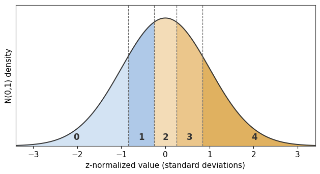
Fig. 4. SAX cuts the standard normal into five equiprobable bands with the four Gaussian breakpoints, so each symbol from 0 to 4 is equally likely on random data

Two design decisions matter here. The z-normalization is what removes a steady drift: constant returns become a flat band of near-identical z-values plus noise, so they symbolize as noise, not as structure. The removal is conditional, not unconditional. Z-normalization strips level and scale, but it does not erase determinacy, so a run whose drift shifts or is sharply asymmetric keeps a shape the measure will read as structure, which is the honest reading rather than a failure. And the breakpoints are computed, not hard-coded. Instead of storing breakpoint tables, the library computes the inverse normal quantile using Acklam's rational approximation. It matches standard SAX tables and agrees with SciPy's quantile to about 1e-12. Building the table is a short loop.

//+------------------------------------------------------------------+
//| Breakpoints = the alphabet-1 equiprobable Gaussian quantiles.    |
//|   b[i] = Phi^-1( (i+1) / alphabet ),  i = 0 .. alphabet-2        |
//|   For alphabet = 3 this is {-0.4307, +0.4307}, matching the      |
//|   standard SAX breakpoint tables exactly.                        |
//+------------------------------------------------------------------+
void CLZSymbolizer::BuildBreakpoints()
  {
   int nb = m_alphabet - 1;
   ArrayResize(m_bp, nb);
   for(int i = 0; i < nb; i++)
      m_bp[i] = Probit((double)(i + 1) / (double)m_alphabet);
  }

The mapping itself lives in the symbolizer's main routine. The excerpt below is the core of it, with the range check trimmed for space: compute the window mean and population standard deviation, guard the flat case where the standard deviation is effectively zero, then map each block mean to the count of breakpoints it clears.

//--- 1) window mean and population std (ddof = 0, SAX convention)
   double mean = 0.0;
   for(int i = 0; i < count; i++)
      mean += series[start + i];
   mean /= (double)count;

   double var = 0.0;
   for(int i = 0; i < count; i++)
     {
      double d = series[start + i] - mean;
      var += d * d;
     }
   var /= (double)count;
   double sd = MathSqrt(var);
   bool   flat = (sd <= 1e-12 * (MathAbs(mean) + 1.0));   // relative flat guard

//--- 3) map each block mean (of the z-normalized window) to a symbol
   for(int s = 0; s < nseg; s++)
     {
      int lo = s * m_paa;
      int hi = lo + m_paa;
      if(hi > count)
         hi = count;

      double blk = 0.0;
      for(int i = lo; i < hi; i++)
         blk += series[start + i];
      blk /= (double)(hi - lo);

      double z = (flat ? 0.0 : (blk - mean) / sd);

      //--- symbol = number of breakpoints at or below z (searchsorted-right).
      //--- breakpoints are ascending, alphabet-1 of them, so 0..alphabet-1.
      int sym = 0;
      for(int k = 0; k < m_alphabet - 1; k++)
         if(z >= m_bp[k])
            sym++;
         else
            break;

      symbols[s] = (uchar)sym;
     }

The flat guard is not cosmetic. A perfectly flat window is maximally predictable, and it should map to a single repeated symbol so the complexity reads near zero. Without the guard, dividing by a standard deviation of zero would produce nonsense, so a flat window is forced to symbol counts around the middle band and reads as regular, which is the correct low-complexity end of the scale.

A worked example makes the mapping concrete. Suppose a short window of returns, after z-normalization, gives the values -1.9, -0.3, 0.1, 0.7 and 2.0. With the five-symbol alphabet the breakpoints sit at -0.84, -0.25, 0.25 and 0.84. The first value falls below every breakpoint and becomes symbol 0, the second lands between the first two as symbol 1, the third and fourth as symbols 2 and 3, and the last clears all four as symbol 4. The window becomes the string 0 1 2 3 4, which the complexity engine then reads. A window whose moves clustered tightly around the mean would instead produce a run of 2s, a low-complexity string, which is exactly the low-information case the measure should flag.

Building the library

The code is organized as four headers under a single include folder, each a small class with one job. The layout follows the same conventions used across the author's other libraries: a boxed header comment on every class and function, private members prefixed with m_, geometric growth for any dynamic array, and a facade that hides the pipeline behind one or two calls while still exposing each stage for testing.

File	Class	Responsibility
LZSymbolizer.mqh	CLZSymbolizer	SAX discretization of a real-valued window into a symbol string
LZComplexity.mqh	CLZComplexity	LZ76 phrase count and its normalized form
LZNCD.mqh	CLZNCD	Normalized Compression Distance between two symbol strings
LZ.mqh	CLZ	Facade: series to efficiency, or two series to a distance

The facade is the entry point most callers use. Its efficiency method takes a price array and a window, and returns the normalized complexity of that window. When the returns flag is set, it converts the slice to log-returns first, which is the market-efficiency reading; otherwise it symbolizes the levels directly, which measures the shape of the price path. Scratch buffers are members, grown once and reused, so repeated calls on a chart do not thrash the allocator.

//+------------------------------------------------------------------+
//| Normalised complexity of one window                              |
//+------------------------------------------------------------------+
double CLZ::Efficiency(const double &price[], int seriesLen,
                       int start, int count, bool useReturns)
  {
   int nsym;
   if(useReturns)
     {
      if(!CLZSymbolizer::LogReturns(price, seriesLen, start, count, m_retA))
         return -1.0;
      int nret = ArraySize(m_retA);
      nsym = m_sym.Symbolize(m_retA, nret, 0, nret, m_symA);
     }
   else
      nsym = m_sym.Symbolize(price, seriesLen, start, count, m_symA);

   if(nsym < 0)
      return -1.0;

   return m_lz.Normalized(m_symA, nsym, m_sym.Alphabet());
  }

The negative return value is the error channel. A window that cannot be built, for example one that contains a non-positive price when returns are requested, yields minus one, and callers treat that as "no reading" rather than as a valid complexity. The indicator uses this to leave a gap in the plot instead of drawing a false zero.

Two conventions run through the code. Every dynamic array grows geometrically rather than one element at a time, because resizing by one inside a loop is quietly quadratic; the buffers double their capacity when they run out and keep it for reuse afterward. And the facade keeps each stage reachable rather than sealed off. The symbolizer, the complexity engine, and the distance are handed back through accessors, so a caller who wants to change the alphabet, read out the raw symbols, or drive the complexity walk on a string of its own can do so without going around the front door. The facade is a convenience, not a wall.

Comparing two windows: Normalized Compression Distance

Complexity measures one window against itself. Normalized Compression Distance, or NCD, measures two windows against each other. The idea is the same compression intuition applied to a pair: if two series are alike, compressing them together costs little more than compressing the larger one alone, because the compressor reuses the structure of the first while packing the second. If they have nothing in common, the joint size is close to the sum. The distance formula captures this:

NCD(x,y) = ( C(xy) - min(C(x),C(y)) ) / max(C(x),C(y))

Here C is a compressed size and xy is the concatenation of the two symbol strings. The value runs from about 0 for identical inputs to about 1 for unrelated ones. The library uses its own LZ76 phrase count as C rather than a real compressor like zlib. That is a deliberate choice. A zlib output length shifts with library version and compression level, which would make an exact cross-check impossible to pin down, whereas the phrase count is a fixed integer function of the string. Because NCD is scale-invariant in C, a constant factor cancels top and bottom, so using a phrase count instead of a byte count changes nothing about the distance.

The figure below shows the measure behaving as it should over many random draws. The self-distance is near zero, a string against a copy with 10 percent of its symbols changed is small, and a string against an unrelated string is large. NCD detects literal shared substructure, which makes it a good tool for asking whether one price window looks like another, not for detecting statistical similarity between two noise processes.

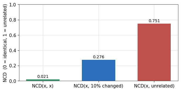
Fig. 5. Normalized Compression Distance is near zero for a string against itself, small for a copy with a tenth of its symbols changed, and large for an unrelated string

The implementation is short. It concatenates the two strings, computes three complexities, and applies the formula, guarding the degenerate case where the larger complexity is zero.

//+------------------------------------------------------------------+
//| NCD(x, y)                                                        |
//+------------------------------------------------------------------+
double CLZNCD::Distance(const uchar &x[], int nx,
                        const uchar &y[], int ny) const
  {
   if(nx <= 0 || ny <= 0)
     {
      Print("CLZNCD::Distance - empty symbol string");
      return -1.0;
     }

//--- concatenation xy
   uchar xy[];
   ArrayResize(xy, nx + ny);
   ArrayCopy(xy, x, 0,  0, nx);
   ArrayCopy(xy, y, nx, 0, ny);

   int cx  = m_lz.Complexity(x,  nx);
   int cy  = m_lz.Complexity(y,  ny);
   int cxy = m_lz.Complexity(xy, nx + ny);

   int cmin = (cx < cy ? cx : cy);
   int cmax = (cx > cy ? cx : cy);
   if(cmax <= 0)
      return 0.0;

   return (double)(cxy - cmin) / (double)cmax;
  }

NCD is a quasi-distance, not a true metric. The distance of a string to itself is small but not exactly zero, because the joint string still opens a phrase or two at the seam between the two copies. The library reports that residual honestly rather than clamping it to zero, which is why the self-distance bar in the figure sits slightly above the axis.

In trading, NCD is best used for template matching on price shape. You symbolize a recent window and a historical window, then compare them with level and scale removed by SAX z-normalization. Because the measure keys on literal shared substrings, it rewards windows that trace a genuinely similar path rather than two windows that merely happen to be equally noisy. That is its strength and its limit at once, and the rest of this section puts it to work.

The demonstration is an analog search. The query is the most recent window of a chart, here 200 bars of EURUSD. Every earlier window of the same length is a candidate, NCD scores each one against the query, and the lowest scores are the nearest analogs, the historical stretches whose symbolized path most resembles today. The script LZ_NCD_AnalogSearch.mq5 does exactly this over 5601 candidate windows, and it keeps the retrieval question and the prediction question strictly apart, because conflating them is how a similarity tool gets mistaken for a forecast.

Retrieval works, and by a clear margin. The three nearest analogs average an NCD of 0.570 against a median of 0.793 across the whole field, so the search really does surface windows whose shape is closer than the run of history, not windows it merely labels closer. The left panel below overlays today against its single nearest analog, both z-normalized so the comparison is the one the measure makes. They share the broad arc, a fall, a long base, a recovery, yet the best match among more than five thousand windows is only 0.55, well short of a copy. That gap is itself a result: an efficient tape does not repeat its own shapes cleanly, so there is no exact precedent to be found, only a loose family resemblance.

The right panel is the control. For each analog, the scan records the forward 20-bar log-return. The three returns are -0.08%, -0.05%, and +0.19%, with no agreement in sign. Their mean (+0.019%) is indistinguishable from a null built from 5,000 random draws (mean +0.006%, sd 0.184%). The resulting z-score is 0.07, dead inside the random band. A shape that looked like today told you nothing about what came next.

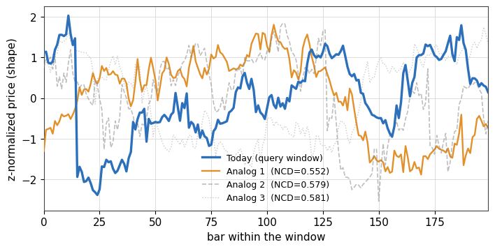
Fig. 6. NCD as a shape search on EURUSD. Left, today's window against its nearest analog among 5601 candidates; the two share the broad arc, but the closest match is only NCD 0.55, so even the nearest historical shape is far from a copy. Right, the forward move after the matched analogs sits at z = 0.07, deep inside the random-window band, so the retrieved shape carries no information about what follows.

So NCD does the job it claims and refuses the job it does not. It retrieves the most similar historical shapes, cleanly and measurably, and it makes no promise about the future once it has. That is the same discipline the efficiency line demands, a descriptive statistic read for what it is rather than pressed into a signal, and it closes the same loop: a market efficient enough to hide a directional edge is also a market that does not hand you a usable precedent for the shape in front of you.

Testing it to death

A complexity library is easy to get subtly wrong and hard to eyeball, so it is verified at three levels before it is trusted on a chart. The philosophy is to check the code against something that does not share its assumptions.

Named facts. The first script asserts values that can be stated without any reference implementation. The complexity of a constant string is 2, the complexity of a period-2 string of length 10 is 3, and the classic Lempel-Ziv example string 0001101001000101 has complexity 6. The SAX breakpoints for alphabet 3 are plus and minus 0.4307, and for alphabet 5 they are the four quantiles at plus and minus 0.8416 and 0.2533. A monotone ramp must map to a non-decreasing symbol sequence, a flat window to a single repeated symbol. This script reports 17 checks passing.

Invariants under randomness. Random tests that assert fixed counts eventually fail on an unlucky draw, so this level asserts orderings that survive the noise, averaged over many draws. A random symbol string scores well above a periodic one. A random walk reads near 1, while a mean-reverting series reads clearly lower because its returns carry serial structure. A trend reads the same as a random walk, confirming that z-normalization strips the drift. Over 10,000 samples the five SAX symbols come out equiprobable to within a fraction of a percent. This script reports 10 checks passing.

An independent cross-check. A Python script recomputes everything the MQL5 side computes, but shares no logic with it. The breakpoints come from scipy's normal quantile rather than Acklam's approximation. The complexity comes from a substring-factorization parse rather than the Kaspar and Schuster index walk. That independent parse was itself validated against the mirror on 4000 random strings before being trusted. An MQL5 script exports a set of deterministic cases, series values written at full double precision, along with the library's own symbols, complexities, and distances. The Python side reads those inputs, computes its own answers, and demands agreement. It reports all 20 cases passing.

The reason for the split between a statement-for-statement mirror and a genuinely independent check is worth stating. The mirror exists so that development can compare numbers line by line while writing the code. The independent check exists so that a shared bug in the algorithm cannot hide, because two different algorithms computing the same integers by different routes is strong evidence the integer is right.

The numbers those scripts print are worth keeping in view. The behavior script measures a random walk at an efficiency near 0.98 and a mean-reverting series near 0.86, a gap of more than a tenth that holds across every random seed. The symbol frequencies on ten thousand Gaussian draws come out as 0.199, 0.203, 0.196, 0.201 and 0.202, within 0.005 of the flat 0.2 the breakpoints promise. None of these are asserted as fixed values, which noise would eventually break; they are asserted as orderings and ranges with measured headroom, the only kind of threshold that survives a random draw.

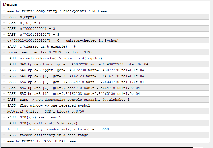
Fig. 7. The Experts tab after a verification script runs, every check passing before the library is trusted on a chart

The efficiency indicator

The indicator plots the efficiency line one reading per bar. Each bar uses the trailing window of closes ending at that bar, converts it to log-returns when the returns mode is on, symbolizes, and stores the normalized complexity. The cost per bar is tiny, a single complexity pass over a few hundred symbols, but a fresh attach still caps how far back it computes so the chart thread is never blocked by the whole history at once.

   for(int i = start; i < last; i++)
     {
      int wstart = i - need + 1;     // window ends at the just-closed bar i
      double e = g_lz.Efficiency(close, rates_total, wstart, need, InpUseReturns);
      g_eff[i] = (e < 0.0 ? EMPTY_VALUE : e);
     }

//--- forming bar mirrors the last closed reading (no half-bar flicker)
   if(last >= 1)
      g_eff[last] = g_eff[last - 1];

Two details keep the plot honest. Only closed bars are scanned, and the forming bar simply mirrors the last closed reading, so the line does not flicker as the current bar ticks. And a window that fails to build writes the plot's empty value rather than a zero, so a genuine gap and a genuine zero never look the same. The arrays inside OnCalculate are indexed oldest to newest, matching the library convention, so no reversal is needed.

The inputs expose the choices that matter. InpWindow sets how many bars each reading spans, InpAlphabet the number of SAX symbols, and InpUseReturns switches between the efficiency reading on returns and the shape reading on levels. InpHistoryBars caps the first-load depth: a fresh attach computes only the most recent stretch and leaves the older bars empty, so the chart thread is never asked to sweep thousands of bars in one pass. The default window of 200 and alphabet of 5 are the same settings used in the market study that follows, so the line you see on a chart and the numbers in that study are the same measure.

Reading the line follows the rule stated at the top. Near 1.0 the recent moves are effectively random. A sustained dip below 1.0 marks a stretch where the moves carry more structure than noise would. What that structure is, and whether it is anything you could trade, is the question the final section answers.

Reading real markets without fooling yourself

Point the measure at a real symbol and a trap springs immediately. Compared against a Gaussian random walk of the same length, EURUSD returns look inefficient: the real efficiency sits well below the walk. Taken at face value, that says the market is predictable. It is not, and the reason is the return distribution.

Real returns are fat-tailed. A window of them, once z-normalized, has most values bunched near the middle with occasional extremes, which is less uniform than a Gaussian window and therefore compresses better and reads as lower complexity. This has nothing to do with predictability. The figure below makes the point with two iid series, one Gaussian and one fat-tailed, built to the same standard deviation. Neither has any serial structure, both are unpredictable by construction, yet the fat-tailed one reads a lower efficiency purely because of its shape.

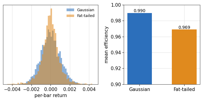
Fig. 8. Two iid series with the same standard deviation; the fat-tailed one reads a lower efficiency than the Gaussian one purely because of its shape, with no predictability behind the drop

So the Gaussian walk is the wrong reference. It differs from a real tape in two ways at once, its distribution and its serial order, and it blames both on inefficiency. Use a second reference that isolates serial structure. Shuffle the symbol's own returns to preserve the distribution while destroying order. The Gaussian-to-shuffled gap is a distribution effect, which is not tradable. The shuffled-to-real gap is a serial-order effect: everything that lives in the order of the returns rather than in their distribution. That bundle is broad. Shuffling destroys autocorrelation, volatility clustering, regime persistence, and any session or seasonal rhythm all at once, so the serial gap holds all of them together, not a clean directional signal. It is the part that could carry exploitable structure, not proof that any of it is exploitable, and the direction test below narrows it further.

The measurement below is EURUSD on the 5-minute timeframe, over 2000 windows of 200 bars each. The walk sits highest, the shuffled real series sits lower by the distribution gap, and the real series sits lower still by the serial gap.

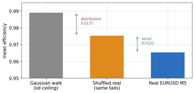
Fig. 9. Decomposing the walk gap on EURUSD M5; the drop from the Gaussian walk to the shuffled real series is the return distribution, and only the smaller drop to the real series is serial structure

One shuffle can land high or low by luck, so the serial gap is judged by a permutation test rather than a single draw. The scan shuffles the returns many times, sweeps each shuffled series, and collects the mean efficiency of each. The spread of those means is the noise band the real mean has to beat. The excerpt below is the heart of the test, shuffling with Fisher-Yates, rebuilding a price path, and sweeping it.

//--- permutation shuffles of the real returns
   double rets0[];
   ArrayResize(rets0, total - 1);
   for(int i = 1; i < total; i++)
      rets0[i-1] = MathLog(close[i] / close[i-1]);

   double shufMeans[];
   ArrayResize(shufMeans, nShuffles);
   double effShuf1[];
   int nShuf1 = 0;
   double rets[];
   ArrayResize(rets, total - 1);
   double shuf[];
   ArrayResize(shuf, total);
   for(int s = 0; s < nShuffles; s++)
     {
      ArrayCopy(rets, rets0);
      for(int i = total - 2; i >= 1; i--)
        { int j = MathRand() % (i + 1); double t = rets[i]; rets[i] = rets[j]; rets[j] = t; }
      shuf[0] = close[0];
      for(int i = 1; i < total; i++)
         shuf[i] = shuf[i-1] * MathExp(rets[i-1]);
      double e[];
      int ne = Sweep(lz, shuf, total, nReadings, need, useReturns, e);
      double m = 0.0;
      for(int i = 0; i < ne; i++)
         m += e[i];
      m /= ne;
      shufMeans[s] = m;
      if(s == 0)
        {
         ArrayCopy(effShuf1, e);
         nShuf1 = ne;
        }
     }

Even a significant serial gap is not yet a directional edge. Volatility clustering, the tendency of large moves to follow large moves, is serial structure that lowers the reading, but it predicts the size of the next move, not its sign. To separate size from direction, the scan runs the whole test a second time at alphabet 2. With two symbols the breakpoint sits at zero, so the symbol is just the sign of the move. Structure that survives the alphabet-2 pass is directional; structure that vanishes in it was volatility, not direction.

Running this for two symbols across two timeframes yields the 2x2 table below. The blue bar is the magnitude pass, the orange bar is the direction pass, and the dashed line marks the z-score of 2 that a result must clear to count as significant.

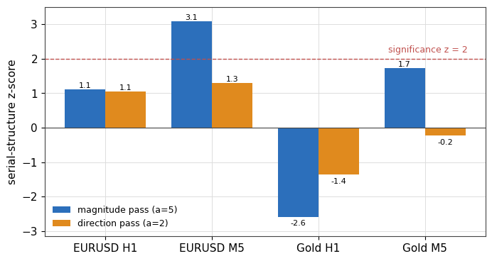
Fig. 10. Serial-structure z-scores for EURUSD and gold at H1 and M5; structure clears the significance line only at M5, and the direction pass never clears it, so nothing directional survives

The pattern is clean. At the hourly timeframe both symbols are efficient: the magnitude z-scores are 1.11 for EURUSD and minus 2.58 for gold, both well inside the shuffle band. At 5 minutes serial structure appears, clearly for EURUSD at z equal to 3.08 and marginally for gold at 1.73. Because both assets are efficient at H1 and both develop structure at M5, the structure is a timeframe effect, the fingerprint of microstructure, not a property of gold or the euro. And in every one of the four cells the direction pass stays below significance, so the M5 structure is volatility clustering, with at most a faint mean-reversion hint in the most liquid pair. There is no directional edge anywhere in this study.

Symbol and timeframe	Magnitude z	Direction z	Reading
EURUSD H1	1.11	1.05	Efficient
EURUSD M5	3.08	1.30	Structure, not directional
Gold H1	-2.58	-1.35	Efficient
Gold M5	1.73	-0.23	Borderline structure

The split behind those z-scores is as telling as the verdicts. On EURUSD M5 the walk gap of about 0.05 breaks into roughly 0.014 of return distribution and 0.010 of serial structure, so most of the apparent inefficiency was never predictability at all, it was fat tails. On gold at the hourly scale the real series actually reads slightly above its own shuffle, a reminder that once the distribution is controlled for, the serial gap can fall on either side of zero. Only the 5-minute cells lift any serial structure above the noise band, and the direction pass then strips even that down to variance. A trader reading the raw efficiency line alone would have seen four markets that all look mildly inefficient; the decomposition shows that none of them offer a sign you could bet on.

Important: the complexity numbers depend on the exact window of history swept, so a rerun on a later window shifts them slightly, and a borderline cell can move across the significance line. Treat the readings as a distribution to be tested against the shuffle null, never as a single number to be trusted on its own.

This is the honest result the tool was built to reach. A naive reading called EURUSD inefficient; the decomposition showed that the bulk of the gap was the fat-tailed return distribution, that the residual was only borderline significant, and that none of it was directional. The value of the measure is diagnostic, telling you what kind of structure a market carries and correctly attributing it, not handing you a signal.

Limitations and honest scope

The measure has real limits, and naming them is part of using it well.

• The efficiency reading on returns is dominated by the return distribution unless it is compared against the shuffle null. Any claim of inefficiency that skips that comparison is measuring fat tails, not predictability.
• Serial structure is not a directional edge. Volatility clustering shows up strongly on short timeframes and predicts variance, not the sign of the next move. The alphabet-2 pass is what tells them apart.
• The readings are window-dependent and should be read as a distribution against a null, not as a single trusted value.
• NCD detects literal shared substructure, so it is suited to comparing the shape of one price window against another, not to finding statistical kinship between two noise processes.
• The complexity walk is O(N^2) in the worst case over the window length. That is negligible for the few-hundred-bar windows used here, but it is not free for very long windows.
• The alphabet size and window length are choices, not universals. A larger alphabet resolves finer structure but needs more data before its symbol frequencies settle, and a longer window smooths the reading at the cost of reacting later. The defaults here suit a few hundred bars and five symbols; a very different market or timeframe may want different ones, and they should be checked against the same shuffle null before they are trusted.
• The measure reads the symbolized series, not the raw returns. The z-normalization across the window, the optional aggregation, and the SAX cut all shape what the complexity engine sees, and on a finite window the symbol frequencies are never perfectly equal. A reading is therefore a statement about the symbols, and the discretization is part of the measurement rather than a neutral window onto the data.
• The reference at 1.0 is a theoretical limit for an infinite random string. On a finite window the noise baseline sits a little below 1.0 and drifts with the alphabet size and window length, which is exactly why the market section compares against a shuffle of the real returns rather than against the flat 1.0 line. The dotted line at 1.0 is an orienting reference, not a calibrated threshold.
• The empirical study here is two symbols on two timeframes, EURUSD and gold at H1 and M5. That is enough to demonstrate the method and the timeframe contrast, not enough to make a general claim about market efficiency. The verdicts are worked examples, not a survey.
• This article defends one tool rather than benchmarking it. Permutation entropy, sample and approximate entropy, Hurst-style exponents, BDS nonlinearity tests, and transfer-entropy approaches all attack the same question from different angles. LZ complexity's advantages here are that its core is parameter-light and it ports cleanly to MQL5, not a demonstrated superiority over those alternatives.

None of this makes the tool weak. It makes it honest. A complexity reading is a strong descriptive statistic and a poor trading signal, and the library is built to let you use the first without mistaking it for the second.

Conclusion

This article built a compact Lempel-Ziv complexity and Normalized Compression Distance library in pure MQL5, wrapped it behind a facade, and shipped an efficiency indicator on top of it. The complexity formula itself takes no parameters, though the pipeline around it makes real choices: an alphabet size, a window length, and whether it reads returns or levels. What it reports is a single number on a fixed scale. More importantly, the article built the discipline to read that number: the shuffle null that separates the return distribution from genuine structure, the permutation test that separates signal from luck, and the alphabet-2 pass that separates volatility from direction. Run against EURUSD and gold, the tool reached an honest verdict, efficient at H1, mild microstructure at M5, no directional edge, and it reached it without fooling itself.

What was built:

• A four-header library: a SAX symbolizer, an LZ76 complexity engine, an NCD distance, and a facade.
• An efficiency indicator that plots one reading per bar with a history-depth guard.
• A three-level verification suite, from named facts to invariants to an independent Python cross-check.
• A market-scan script that decomposes the reading into distribution, serial, and directional parts against the right nulls.
• An NCD analog search that retrieves a window's nearest historical shapes and shows, against a random null, that a matched shape is not predictive.

#	Filename	Type	Description
1	LZSymbolizer.mqh	Include	SAX discretization of a window into a symbol string
2	LZComplexity.mqh	Include	LZ76 phrase count and normalized complexity
3	LZNCD.mqh	Include	Normalized Compression Distance between two symbol strings
4	LZ.mqh	Include	Facade: series to efficiency, or two series to a distance
5	LZ_Efficiency.mq5	Indicator	Rolling market-efficiency line in a subwindow
6	LZ_Test_Complexity.mq5	Script	Unit tests on named facts
7	LZ_Test_Behavior.mq5	Script	Behavior tests: invariants under randomness
8	LZ_Export_Crosscheck.mq5	Script	Export deterministic cases for the Python cross-check
9	LZ_Scan_Market.mq5	Script	Real-market scan with distribution, serial, and direction nulls
10	LZ_NCD_AnalogSearch.mq5	Script	NCD shape search: nearest historical analogs plus the predictiveness control
11	lz_crosscheck.py	Python	Independent cross-check: scipy quantiles and a substring-factor parse
12	lz_ref.py	Python	Statement-for-statement mirror of the library
13	MQL5.zip	Archive	Archive with all the files above, ready to unpack into the terminal data directory so each file lands in its correct location