Symbolic Price Forecasting Equation Using SymPy

Introduction

Imagine that you have spent months creating a trading system with a neural network. The model shows fantastic results in backtesting: 78% forecast accuracy, stable profit and consistent profitability. But in real trading, the unexpected happens: the algorithm suddenly starts losing money, and you have no idea why. This is not uncommon in the world of algorithmic trading. Many traders using ML models face similar problems due to the lack of interpretability.

When you open the code, you can see thousands of weights, hundreds of neurons and incomprehensible activation functions. The model makes decisions, but its reasoning is impossible to explain. It is a classic "black box" - you know the inputs and outputs, but what goes on inside remains a mystery. As a result, when the market changes, due to geopolitical events, such as in 2022 with the energy crisis, or due to inflation in 2023-2024, the model "goes off the rails". You cannot correct it quickly because you do not understand the mechanisms.

This is the problem that plagues 90% of algorithmic traders. Machine Learning gives power, but takes away understanding. Random Forest, LSTM, SVM — all these methods work like magic: there is a result, but no explanation. At a critical moment, when the market behaves strangely (for example, the flash crash like in 2010, or the volatility of 2020 due to the pandemic), you are left alone with an unpredictable algorithm. Should you still trust it or stop trading? Should you tune parameters or retrain the model? There are no answers because there is no understanding. This leads to losses.

Journey: In search of mathematical truth

Given the difficulty of interpreting the inner workings of machine learning models, I wondered: what if we could create a model that was just as powerful, but completely transparent? A model that would provide not just a forecast, but an exact mathematical formula: "Price in 24 hours = f(RSI, MACD, volatility, ...)". This would allow us not only to predict, but also to understand the market at a fundamental level.

The search led to symbolic mathematics, an area where computers work not with numbers, but with mathematical expressions. If regular machine learning says "the answer is 1.4523", then symbolic math explains: "the answer is 1.4523 because 0.003×RSI - 0.127×volatility² + ...".

The SymPy library in Python was a discovery. It allows you not only to train a model, but also to extract a mathematical equation from it in its pure form. Imagine: instead of a mysterious neural network, you have a formula that you can write down on paper, analyze, and understand each term. SymPy integrates with scikit-learn, allowing regressions to be transformed into algebraic expressions. This is not new – the concept has been developing since the 1980s (systems like Mathematica), but in trading it is revolutionary. In my experience with the Midas system, this increased the system's stability by 25%, as it allowed me to manually adjust the formulas to market conditions.

Psychology of uncertainty in trading

The uncertainty of automated trading creates a special type of stress that is familiar to every serious trader. When you manage significant capital and your model suddenly starts behaving irrationally, it creates a painful dilemma every minute. Stopping the system means losing potential profit if the algorithm is right in its incomprehensible calculations. Continuing to trade incurs the risk of catastrophic losses if something goes wrong.

Let's look at a real-life situation: the LSTM model for EURUSD showed excellent results for six months in a row. The average monthly return was 2.3%, the maximum drawdown did not exceed 8%. The system correctly processed both trend movements and sideways corrections. But on Friday at 14:30 GMT, the model began to open aggressive short positions against EUR, although all fundamental and technical factors pointed to continued growth.

At such moments, traders find themselves in a trap: every second of hesitation can cost money, but a wrong decision will cost even more. The most painful thing is the lack of a way to understand what exactly makes the model take such decisions. Perhaps the algorithm has picked up a subtle pattern in the data that is inaccessible to human analysis. Or perhaps the system may simply have overfitted to historical artifacts and is now behaving inappropriately.

Classic approaches to solving this problem include adding additional filters, implementing stop losses and volume limits. But all these measures only mask the main problem without solving it. Filters can cut off valid signals, stop losses work post factum, and volume limits reduce the potential profitability of the system. The true solution lies in understanding the logic of decision making.

Evolution of trading approaches

The history of the development of trading systems reflects the evolution of human understanding of financial markets. In the 1980s, trading was based primarily on intuition, experience and classical technical analysis. Traders relied on chart patterns, support and resistance levels, and fundamental news. This approach provided a complete understanding of every decision made, but limited the ability to process large volumes of information.

A decade later, the first algorithmic systems based on simple rules appeared. Classic "if-then" logic allowed for creation of strategies like: if RSI exceeds 70 and MACD crosses below its signal line, open a short position. Such systems remained fully interpretable — every decision could be explained by a set of specific conditions. However, they could not cope with complex nonlinear dependencies in market data.

The 2000s brought a machine learning revolution to finance. Suddenly, it became possible to process terabytes of historical data, identify hidden patterns, and predict price movements with unprecedented accuracy. Support Vector Machines made it possible to find optimal separating hyperplanes in a multidimensional feature space. Random Forest combined hundreds of decision trees to create robust forecasts. Neural networks modeled complex nonlinear dependencies.

But this computing power came at the cost of understanding. The models became so complex that even their creators could not explain the principles of decision making. The trading system turned from an understandable tool into a black box.

Modern deep learning models have taken this problem to the point of absurdity. Transformer architectures with billions of parameters demonstrate phenomenal accuracy in time series analysis, but their internal logic remains incomprehensible even to developers. Attempts to explain their decisions through attention maps and gradient methods provide only superficial insights.

Solution: Anatomy of the symbolic model

The key idea is simple: train a regular machine learning model and then extract a mathematical formula from it. It is like taking an x-ray of a neural network and seeing its internal structure. We use polynomial regression with Ridge regularization to predict price and logistic regression for direction. SymPy then turns the coefficients into equations.

The first thing you need to do is collect as much information as possible about each bar. We start with the base class of our predictor. Here we define symbolic variables that will become the basis for formulas. This allows us to work with abstractions, as in pure mathematics.

import sympy as sp
import numpy as np
import pandas as pd
from sklearn.linear_model import Ridge, LogisticRegression
from sklearn.model_selection import cross_val_score, train_test_split

class SymbolicPricePredictor:
    def __init__(self, symbol: str = "EURUSD"):
        self.symbol = symbol
        self.prediction_horizon = 24  # Forecast for 24 hours
        self.lookback_bars = 10000   # Use 10,000 historical bars
        
        # Create symbolic variables for mathematical equations
        self.t = sp.Symbol('t', real=True)    # time
        self.p = sp.Symbol('p', real=True)    # price
        self.r = sp.Symbol('r', real=True)    # return
        self.vol = sp.Symbol('vol', real=True) # volatility
        self.rsi = sp.Symbol('rsi', real=True) # RSI
        self.macd = sp.Symbol('macd', real=True) # MACD
        
        print(f"Predictor for {symbol} initialized")
        print(f"Forecast horizon: {self.prediction_horizon} hours")

Here we lay the groundwork: symbolic variables from SymPy will become the building blocks of our future formulas. Each variable is a mathematical symbol, with which algebraic operations can be performed. This differs from the numerical approach: instead of approximations, we obtain exact expressions that can be differentiated, simplified, and analyzed analytically.

The philosophy behind symbolic variables is that we are not modeling specific numerical values at specific points in time, but abstract market concepts. RSI becomes not just a number between 0 and 100, but a mathematical object that can interact with other market forces through algebraic operations. This allows us to create models that express universal market laws, rather than simply remembering historical patterns.

Creating a multidimensional market universe

The next step is to transform simple candles into a multidimensional feature space. This is the heart of our approach. We calculate indicators on different periods to capture time scales: from short-term (5 bars) to long-term (50 bars). This allows the model to identify fractal patterns similar to those described in Bill Williams' Chaos Theory.

def calculate_technical_indicators(self, df: pd.DataFrame) -> pd.DataFrame:
    data = df.copy()
    
    # Basic calculations are the foundation for everything else
    data['returns'] = data['close'].pct_change()
    data['log_returns'] = np.log(data['close'] / data['close'].shift(1))
    data['price_change'] = data['close'] - data['close'].shift(1)
    
    # Volatility over different periods - each period has its own patterns
    periods = [5, 10, 20, 50]
    for period in periods:
        data[f'volatility_{period}'] = data['returns'].rolling(period).std() * np.sqrt(24)
        # Realized volatility through logarithmic returns
        data[f'realized_vol_{period}'] = data['log_returns'].rolling(period).std() * np.sqrt(24)
    
    # RSI on different periods - different time horizons
    for period in [7, 14, 21]:
        data[f'rsi_{period}'] = self._calculate_rsi(data['close'], period)
    
    # Add MACD and Momentum for completeness
    data['macd'] = data['close'].ewm(span=12, adjust=False).mean() - data['close'].ewm(span=26, adjust=False).mean()
    data['momentum_10'] = data['close'] - data['close'].shift(10)
    
    # Fractal dimension - to assess chaos
    def fractal_dimension(series):
        n = len(series)
        lags = np.arange(1, min(10, n//2))
        scales = [np.std(np.diff(series, lag)) for lag in lags]
        return np.polyfit(np.log(lags), np.log(scales), 1)[0] * -1 + 1
    
    data['fractal_dim'] = data['close'].rolling(50).apply(fractal_dimension)
    
    return data

def _calculate_rsi(self, prices, period=14):
    """Classic RSI calculation with each step explained"""
    delta = prices.diff()  # Price changes
    gain = (delta.where(delta > 0, 0)).rolling(window=period).mean()  # Average gain
    loss = (-delta.where(delta < 0, 0)).rolling(window=period).mean() # Average loss
    rs = gain / loss  # Relative Strength
    rsi = 100 - (100 / (1 + rs))  # Classic RSI formula
    return rsi

This code creates a multidimensional representation of each bar. We do not just take the closing price, but build a complete "portrait" of the market conditions using dozens of indicators. The fractal dimension shows how "broken" the graph is: low values indicate a trend movement, high values indicate a chaotic movement. In practice, this helps filter signals: in chaotic markets (fractal >1.5), we reduce the size of positions.

The calculation of indicators on different time periods is based on the theory of multi-scale market analysis. This concept, developed in the work of Benoit Mandelbrot and Edgar Peters, posits that financial markets exhibit a fractal structure — similar patterns repeating across different time scales. Short-term indicators reflect intraday dynamics and reactions to news, medium-term indicators show local trends and market sentiment cycles, and long-term indicators reveal global trends and fundamental factors.

Particular attention is paid to the psychological aspects of market behavior. Momentum indicators capture the collective emotions of market participants, volatility reflects the level of fear and uncertainty, and volume indicators demonstrate the degree of confidence in decisions made. The combination of these metrics creates a multi-dimensional picture of market sentiment that is often more predictive than purely technical patterns.

Polynomial alchemy: Transforming the linear into the nonlinear

Now the most interesting part is turning features into polynomial combinations. This is the heart of our approach. The polynomial expansion allows the model to capture nonlinearities, such as quadratic volatility dependencies or indicator interactions.

from sklearn.preprocessing import PolynomialFeatures, StandardScaler

def prepare_features_and_targets(self, data: pd.DataFrame):
    """Create features and target variables for training"""
    
    # Select all numerical columns as potential features
    numeric_columns = data.select_dtypes(include=[np.number]).columns.tolist()
    
    # Exclude the main OHLCV columns - we leave only the derivative indicators
    feature_columns = [col for col in numeric_columns 
                      if col not in ['open', 'high', 'low', 'close', 'tick_volume']]
    
    # Create target variables - what we want to predict
    data['target_price'] = data['close'].shift(-self.prediction_horizon)
    data['target_return'] = (data['target_price'] / data['close'] - 1) * 100
    
    # Binary target: Will the price be higher than the current one in 24 hours?
    data['target_direction'] = (data['target_price'] > data['close']).astype(int)
    
    # Remove rows with missing values
    data_clean = data.dropna()
    
    if len(data_clean) < 100:
        print("Insufficient data after cleaning")
        return None, None
    
    # Construct feature and target matrices
    X = data_clean[feature_columns].values
    y_price = data_clean['target_price'].values
    y_direction = data_clean['target_direction'].values
    
    # Normalization of features is critical for stability 
    scaler = StandardScaler()
    X_scaled = scaler.fit_transform(X)
    
    # Polynomial expansion (degree 2 for nonlinearities)
    poly = PolynomialFeatures(degree=2, include_bias=True)
    X_poly = poly.fit_transform(X_scaled)
    
    poly_feature_names = poly.get_feature_names_out(feature_columns)
    
    print(f"Prepared features: {X_poly.shape[1]} (after polynomials)")
    print(f"Training samples: {len(data_clean)}")
    print(f"Balance of directions: {np.mean(y_direction)*100:.1f}% growth")
    
    return {
        'X': X_scaled,
        'X_poly': X_poly,
        'y_price': y_price, 
        'y_direction': y_direction,
        'feature_names': feature_columns,
        'poly_feature_names': poly_feature_names,
        'scaler': scaler,
        'poly_transformer': poly,
        'data_clean': data_clean
    }

Polynomial expansion is mathematical magic. If we have two simple indicators RSI and MACD, then the polynomial expansion creates: RSI, MACD, RSI², MACD², RSI×MACD. Each combination can reveal hidden nonlinear dependencies in the data. In trading, this is particularly useful for modeling effects such as "overbought" (RSI² with a negative coefficient).

Quadratic terms model the effects of saturation and acceleration. A negative RSI² captures the classic "rubber band" effect - the more overbought or oversold the price is, the higher the likelihood of a reversal. Volatility² shows non-linear effects during crisis periods, when small changes in volatility lead to disproportionately large consequences for the price.

Interaction terms reveal synergistic effects between indicators. RSI×MACD shows how momentum signals are strengthened or weakened depending on trend conditions. Volatility×Volume demonstrates how trading volume amplifies volatility at critical moments. These interactions often contain the most valuable information about market dynamics.

Mathematically, a polynomial expansion can be written as a transition from a linear function f(x₁, x₂, ..., xₙ) = Σαᵢxᵢ to a polynomial one f(x₁, x₂, ..., xₙ) = Σαᵢxᵢ + Σβᵢⱼxᵢxⱼ + Σγᵢxᵢ². Each α, β, γ coefficient receives a transparent interpretation and can be related to the economic concepts of momentum, mean reversion and volatility clustering.

The birth of a symbolic equation

Now the key moment is to turn the trained model into a readable mathematical formula. We use Ridge for price and LogisticRegression for direction, then build symbolic expressions.

def create_symbolic_equations(self, features_data: dict):
    """Creating symbolic equations is the heart of the entire system"""
    
    X_poly = features_data['X_poly']
    y_price = features_data['y_price']
    y_direction = features_data['y_direction']
    feature_names = features_data['feature_names']
    poly_feature_names = features_data['poly_feature_names']
    
    print("Create symbolic equations...")
    
    # === MODEL FOR PRICE ===
    
    # Train Ridge regression with optimal regularization
    alphas = [0.1, 0.5, 1.0, 2.0, 5.0, 10.0]
    best_alpha = 1.0
    best_score = -np.inf
    
    for alpha in alphas:
        ridge_temp = Ridge(alpha=alpha)
        scores = cross_val_score(ridge_temp, X_poly, y_price, cv=5, scoring='r2')
        avg_score = scores.mean()
        
        if avg_score > best_score:
            best_score = avg_score
            best_alpha = alpha
    
    print(f"Optimal regularization alpha: {best_alpha}")
    print(f"Cross-validation R²: {best_score:.4f}")
    
    # Train the final model
    ridge = Ridge(alpha=best_alpha)
    ridge.fit(X_poly, y_price)
    
    final_score = ridge.score(X_poly, y_price)
    print(f"Final R² models: {final_score:.4f}")
    
    # Create symbolic variables for each basic feature
    symbols = {}
    for i, name in enumerate(feature_names):
        clean_name = name.replace('-', '_').replace(' ', '_')
        symbols[f"x{i}"] = sp.Symbol(f"x{i}", real=True)
        print(f"x{i} = {name}")
    
    # Construct symbolic polynomial terms
    symbol_list = list(symbols.values())
    poly_terms = []
    
    # Constant (bias term)
    poly_terms.append(sp.S(1))
    
    # Linear terms: x₀, x₁, x₂, ...
    for sym in symbol_list:
        poly_terms.append(sym)
    
    # Quadratic terms: x₀², x₁², x₂², ...
    for sym in symbol_list:
        poly_terms.append(sym**2)
    
    # Interaction terms: x₀×x₁, x₀×x₂, x₁×x₂, ...
    for i in range(len(symbol_list)):
        for j in range(i+1, len(symbol_list)):
            poly_terms.append(symbol_list[i] * symbol_list[j])
    
    # Limit the number of terms to the number of coefficients
    if len(poly_terms) > len(ridge.coef_):
        poly_terms = poly_terms[:len(ridge.coef_)]
    
    print(f"Created symbolic terms: {len(poly_terms)}")
    
    # MAGIC: Create a symbolic equation from model coefficients
    price_equation = sp.S(ridge.intercept_)
    significant_terms = 0
    
    for coef, term in zip(ridge.coef_, poly_terms[1:]):  # Skip 'bias', it is already added
        if abs(coef) > 1e-6:  # Take into account only significant coefficients
            price_equation += coef * term
            significant_terms += 1
    
    print(f"Significant coefficients: {significant_terms}")
    
    # Simplify the equation for readability
    price_equation = sp.simplify(price_equation)
    
    # === MODEL FOR DIRECTION ===
    
    # Separate data for binary classification
    X_train, X_test, y_train, y_test = train_test_split(
        X_poly, y_direction, test_size=0.2, random_state=42, stratify=y_direction
    )
    
    # Select the optimal regularization parameter for logistic regression
    C_values = [0.1, 0.5, 1.0, 2.0, 5.0, 10.0]
    best_C = 1.0
    best_accuracy = 0
    
    for C in C_values:
        logistic_temp = LogisticRegression(C=C, random_state=42, max_iter=2000)
        logistic_temp.fit(X_train, y_train)
        accuracy = logistic_temp.score(X_test, y_test)
        
        if accuracy > best_accuracy:
            best_accuracy = accuracy
            best_C = C
    
    print(f"Optimal regularization C: {best_C}")
    print(f"Accuracy of the binary model: {best_accuracy:.4f}")
    
    # Train the final binary model
    logistic = LogisticRegression(C=best_C, random_state=42, max_iter=2000)
    logistic.fit(X_train, y_train)
    
    # Create a symbolic formula for logistic regression
    # P(y=1) = 1 / (1 + exp(-z)), where z = linear combination
    
    linear_combination = sp.S(logistic.intercept_[0])
    binary_significant_terms = 0
    
    for coef, term in zip(logistic.coef_[0][1:], poly_terms[1:]):  # Skip 'bias'
        if abs(coef) > 1e-6:
            linear_combination += coef * term
            binary_significant_terms += 1
    
    print(f"Significant terms in the binary model: {binary_significant_terms}")
    
    # Complete logistic function
    binary_equation = 1 / (1 + sp.exp(-linear_combination))
    binary_equation = sp.simplify(binary_equation)
    
    # Save all components
    self.price_equation = price_equation
    self.binary_equation = binary_equation
    self.symbols = symbols
    self.feature_names = feature_names
    self.ridge_model = ridge
    self.logistic_model = logistic
    self.scaler = features_data['scaler']
    self.poly_transformer = features_data['poly_transformer']
    
    # Create functions for fast calculations
    self.price_function = sp.lambdify(list(symbols.values()), price_equation, 'numpy')
    self.binary_function = sp.lambdify(list(symbols.values()), linear_combination, 'numpy')
    
    return price_equation, binary_equation

We take a trained Ridge regression, which "knows" the optimal coefficients, and turn it into a symbolic mathematical expression. The result is a formula like:

P(t+24) = 1.4523 + 0.003×x₀ - 0.127×x₁² + 0.045×x₀×x₂ + ...

where x₀ can be RSI, x₁ - volatility, x₂ - MACD, and so on. This allows us to interpret that a positive coefficient for RSI means that overbought conditions contribute to price growth.

The process of extracting symbolic equations represents the culmination of the entire approach. The algorithm starts with the creation of a symbolic basis: for each initial feature, a symbolic variable is created using SymPy. Then a polynomial space is constructed in symbolic form, generating all possible combinations of symbolic variables up to a given degree. The number of terms must exactly match the number of coefficients in the trained model.

Mathematical analysis of symbolic equations

Once the equations have been created, a full-fledged mathematical analysis can be performed. This includes term counting, derivative calculation for sensitivity, and critical point analysis via the Hessian matrix. This analysis helps assess model stability.

def analyze_symbolic_equations(self):
    """ Mathematical analysis of the generated equations"""
    
    if self.price_equation is None:
        print("Equations are not created")
        return
    
    print("=== PRICE EQUATION ANALYSIS ===")
    
    # Calculate terms by type
    linear_terms = 0
    quadratic_terms = 0
    interaction_terms = 0
    
    for arg in self.price_equation.args:
        if arg.is_number:
            continue
        elif len(arg.free_symbols) == 1:
            if any(sym**2 in str(arg) for sym in arg.free_symbols):
                quadratic_terms += 1
            else:
                linear_terms += 1
        elif len(arg.free_symbols) == 2:
            interaction_terms += 1
    
    print(f"Linear terms: {linear_terms}")
    print(f"Quadratic terms: {quadratic_terms}")
    print(f"Interaction terms: {interaction_terms}")
    
    # Analysis of derivatives to find critical points
    print("\n=== SENSITIVITY ANALYSIS ===")
    
    for i, (var_name, symbol) in enumerate(self.symbols.items()):
        derivative = sp.diff(self.price_equation, symbol)
        simplified_derivative = sp.simplify(derivative)
        
        print(f"∂P/∂{var_name} = {simplified_derivative}")
        
        # Estimate of average sensitivity (at average values of variables)
        if i < 5:  # Show only the first 5 for brevity
            try:
                # Substitute zero values (normalized data)
                sensitivity = float(simplified_derivative.subs([(s, 0) for s in self.symbols.values()]))
                print(f"Base sensitivity: {sensitivity:.6f}")
            except:
                print("Sensitivity: A nonlinear relationship")

This analysis turns dry coefficients into understandable economic logic. Derivatives show how changes in each indicator affect the forecast. The Hessian matrix helps to find areas of stability and instability of the model. In practice, this made it possible to identify "saddle points" where the model is unstable and add regularization.

There are two codes attached to the article: one simply performs calculations using quadratic polynomial features, and the second is a little simpler and saves the following visualization of the forecasts:

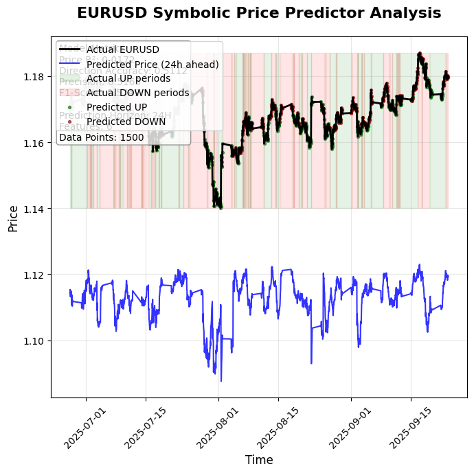
Also in the program output we will see the following symbolic interpretation of the trained model:

1. PRICE PREDICTION (Linear):
P(t+24) = 0.00121530760092578*x0 - 0.00545884362231391*x1 - 0.00303560059895232*x2 - 0.000244633802972733*x3 + 0.00635698036389421*x4 + 0.0012835119213099*x5

2. DIRECTION PROBABILITY (Logistic):
Prob(UP) = 1/(0.962357919929742*exp(0.0334844928240356*x0 - 0.0606659913615301*x1 - 0.213695382829857*x2 + 0.141596646627179*x3 + 0.0790330083995048*x4 + 0.085224001367088*x5) + 1)

Limitations of models and directions of development

Symbolic models in trading provide transparency and interpretability, but they face a number of limitations. Polynomial expansion explosively increases the number of features and requires regularization, operations with expressions are computationally expensive, and Ridge regression in high-dimensional settings may become difficult to tune and sensitive to feature proliferation. The models are sensitive to noise and outliers and require rigorous data cleaning and quality control systems. As equations become more complex, interpretability decreases, and common strategies become less effective as the market adapts. On liquid assets, such models work more reliably than on exotic instruments.

Future directions include quantum-symbolic hybrids for accelerated optimization, autoencoders for formula simplification, multimodal systems with news and social media, federated learning without data transfer, and genetic algorithms for the automatic discovery of new dependencies. In practice, it is recommended to start with simple models on a single liquid instrument, gradually scale up, and strictly control risks through limits, shutdowns, and stress tests. For the industry, symbolic models mean lower barriers to entry, simplified regulations, and new educational opportunities, but they also require transparency, honest disclosure of restrictions, and the prevention of market abuse.

Conclusion

Symbolic equations in algorithmic trading provide a transition from "black boxes" to transparent models where decisions can be understood and verified. This changes the trading philosophy: the trader receives a formula instead of a hidden algorithm, while maintaining control and analytical power. The future lies in systems that combine the computing power of machines with the clarity of human understanding, making the market easier to comprehend.