Neural network trading EA based on PatchTST

Introduction

Remember the time when an overbought RSI meant a correction was imminent, and the MACD clearly showed a trend change? Those days are in the past. Modern markets have become too complex for simple mathematical indicators. Algorithmic traders are eating up the lion's share of profits using machine learning, while retail traders continue to rely on tools that are half a century old.

The death of traditional indicators: Anatomy of failure

To understand the scale of the problem, let's look at the statistics. In the 1990s, a simple strategy based on moving average crossovers delivered a 65–70% win rate on major currency pairs. By 2010, this figure had fallen to 52%. Today it hovers around the level of random chance - about 50%.

The reason does not lie in math. The problem lies in the market’s ability to adapt. When millions of traders use the same signals, the market itself begins to take them into account. This creates a feedback loop: the indicator becomes a self-refuting prophecy. Jim Simons once compared this to a herd of camels in the desert: one camel could live off an oasis for a long time, but a huge herd would quickly drain it dry and be thirsty again.

Moreover, modern markets are exposed to factors that did not exist when RSI and MACD were created. High-frequency trading creates microstructural noise that traditional indicators interpret as false signals. Algorithmic funds with multi-billion dollar assets can artificially create patterns, luring retail traders into traps.

Traditional indicators are based on linear assumptions about market behavior. RSI suggests that extreme values lead to a pullback. Moving averages assume that the price tends to move towards an average value. MACD is based on the idea that short-term trends interact predictably with long-term ones. All of these assumptions worked in less efficient markets of the past, but fail in the context of modern algorithmic trading.

Neural networks: A first attempt at evolution

The first generation of traders, recognizing the limitations of technical analysis, turned to simple neural networks. Multilayer perceptrons of the 1990s seemed revolutionary. They could find nonlinear relationships that eluded linear indicators.

However, these systems also had fundamental flaws. Simple neural networks could not effectively process data sequences. They looked at each bar in isolation, losing the context of the time dynamics. This was particularly critical for financial markets, where current price movements are inextricably linked to previous events.

Recurrent neural networks (RNNs) and LSTMs partially solved this problem, but brought new challenges. The vanishing gradient problem made learning on long sequences virtually impossible. Financial markets require analysis of hundreds, sometimes thousands, of historical bars to make an informed decision.

LSTMs performed best on sequences up to 50-100 elements, but began to lose efficiency on longer time series. The problem was in the architecture - the information had to pass through many intermediate states, losing relevance along the way. For financial data, where an event a week ago could be critical to the current forecast, such limitations were unacceptable.

Transformers: Breakthrough and obstacles

The revolution began in 2017 with the publication of the article "Attention Is All You Need". Transformers have revolutionized sequence processing in NLP, but their application to financial time series has encountered significant hurdles.

The main problem is computational complexity. The attention mechanism requires computing correlations between each pair of elements in the sequence. For a sequence of length N, this gives O(N²) operations. When N = 1000 bars (which is the minimum for serious analysis), the number of operations reaches a million. Each operation involves a high-dimensional matrix multiplication, making the computation extremely resource-intensive.

Moreover, traditional transformers were designed for discrete tokens — words in a text. Financial data are continuous time series with a complex internal structure. Simply applying transformers to price data ignores this specificity. Tokenization by individual bars loses important information about local patterns within short time windows.

Attempts to adapt vanilla transformers for finance have encountered the problem of overfitting. The model easily memorized specific sequences from training data, but could not generalize knowledge to new market situations. This was especially evident during periods of high volatility or structural market changes.

This is where PatchTST comes in — an architecture that revolutionizes how neural networks should analyze financial time series. It is not merely another transformer, but a specially adapted system that understands the nature of market data and works with it like a true professional trader.

The Patch concept: From pixels to bars

The idea of patches came from computer vision. Vision Transformer (ViT) breaks an image into square patches, each of which is treated as a separate token. PatchTST applies a similar principle to time series, but with a deep understanding of financial data.

Each patch in PatchTST represents a segment of 16 consecutive bars. This is not a random choice. Volatility analysis shows that 16 bars is the optimal length to capture local price movement patterns while maintaining computational efficiency. Patterns such as "head and shoulders", "flags" or "pennants" usually develop in these time windows.

Within each patch, the model sees the microstructure of the movement: how the opening price relates to the closing price, what the highs and lows were, how the volume changed. Between patches, the model tracks macrotrends: trend developments, changes in market sentiment, and cyclical patterns. This hierarchical representation allows for simultaneous analysis of short-term tactical options and the long-term strategic picture.

Multichannel architecture: Capturing more dimensions

Unlike simple systems that analyze only the closing price, PatchTST works with multi-channel data. The basic implementation uses two channels - the price change channel represents the normalized difference between the closing and opening prices, and the volume channel contains logarithmically normalized tick volume.

This approach allows the model to see not only "what happened" (price movement), but also "with what force" (volume activity). High volume with little price movement signals that large players are accumulating positions. A sharp move on low volume may indicate a technical breakout without fundamental support, foreshadowing a quick pullback.

Dual-channel architecture creates a rich information space. The model learns to associate certain combinations of price movements and volumes with future outcomes. For example, a gradual decrease in volumes while the price rises often precedes a trend reversal. A spike in volume at a breakout of an important level confirms the strength of the movement.

Attention mechanism in finance

The attention mechanism in PatchTST works differently than in language models. Instead of analyzing semantic relationships between words, it looks for temporal correlations between market events. Imagine the situation: a morning gap down often leads to a recovery move in the afternoon. Traditional indicators cannot capture such long-term relationships.

The PatchTST attention mechanism automatically detects these patterns and assigns them appropriate weights. If the model notices that a certain combination of volume and price action in the morning hours correlates with an evening rally, it will pay special attention to morning patterns when forecasting the evening move.

The multi-headed attention structure allows the model to simultaneously track different types of dependencies. One head may focus on short-term intraday patterns, another on weekly cycles, and a third on correlations between price and volume. Each head develops its own "expertise", and their joint work creates a comprehensive understanding of the market.

Deep dive into implementation

In this article, we will walk you through the entire process of creating a trading robot: from writing the neural network architecture to the final EA, ready for real trading. Every line of code will be explained, every decision justified.

First, let’s implement matrix operations in MQL5. 

struct Matrix {
    double data[];
    int rows, cols;
    
    void Init(int r, int c) {
        rows = r; cols = c;
        ArrayResize(data, r * c);
        ArrayInitialize(data, 0.0);
    }
    
    double Get(int r, int c) { 
        if(r < 0 || r >= rows || c < 0 || c >= cols) return 0.0;
        return data[r * cols + c]; 
    }
    
    void Set(int r, int c, double val) { 
        if(r < 0 || r >= rows || c < 0 || c >= cols) return;
        data[r * cols + c] = val; 
    }
    
    void Random(double scale = 0.1) {
        for(int i = 0; i < ArraySize(data); i++)
            data[i] = (MathRand() / 32767.0 - 0.5) * 2.0 * scale;
    }
}

This structure becomes the basis for all calculations in our neural network. Checking array boundaries is critically important - a single out-of-bounds error can bring down the entire terminal. The Random function deserves special attention. Initializing the weights to a uniform distribution with scale 0.1 provides a good starting point for training. Too large initial weights lead to saturation of activation functions, too small ones lead to slow convergence.

Balancing classes: Handling market imbalance

Financial markets are inherently unbalanced. Periods of calm trading make up 70-80% of the time, strong movements occur rarely. Without compensating for this imbalance, the model will learn to predict only a "neutral" market state.

struct ClassWeights {
    double strong_bull, weak_bull, neutral, weak_bear, strong_bear;
    
    void UpdateWeights(int &counts[]) {
        int total = counts[0] + counts[1] + counts[2] + counts[3] + counts[4];
        if(total == 0) return;
        
        strong_bear = (counts[0] > 0) ? (double)total / (5 * counts[0]) : 1.0;
        weak_bear = (counts[1] > 0) ? (double)total / (5 * counts[1]) : 1.0;
        neutral = (counts[2] > 0) ? (double)total / (5 * counts[2]) : 1.0;
        weak_bull = (counts[3] > 0) ? (double)total / (5 * counts[3]) : 1.0;
        strong_bull = (counts[4] > 0) ? (double)total / (5 * counts[4]) : 1.0;
    }
    
    double GetWeight(double target) {
        if(target > 0.7) return strong_bull;
        if(target > 0.6) return weak_bull;
        if(target > 0.4) return neutral;
        if(target > 0.3) return weak_bear;
        return strong_bear;
    }
};

The algorithm is simple: the less frequently a class occurs, the more weight it receives during training. This forces the model to pay more attention to rare but profitable market moves. The classification into five categories provides sufficient granularity for trading decisions without overloading the model with excessive complexity.

Patch embedding: Transforming data into neural network-friendly vectors

The PatchEmbedding structure is a bridge between raw market data and the model's internal representation. Each 16-bar patch is converted into a 128-dimensional vector.

struct PatchEmbedding {
    Matrix patch_weights;
    Matrix position_embedding;
    
    void Init() {
        patch_weights.Init(PATCH_SIZE * 2, HIDDEN_SIZE);
        patch_weights.Random(0.1);
        
        int max_patches = INPUT_BARS / PATCH_SIZE + 1;
        position_embedding.Init(max_patches, HIDDEN_SIZE);
        
        for(int pos = 0; pos < max_patches; pos++) {
            for(int i = 0; i < HIDDEN_SIZE; i++) {
                double angle = pos / MathPow(10000.0, 2.0 * (i / 2) / HIDDEN_SIZE);
                position_embedding.Set(pos, i, (i % 2 == 0) ? MathSin(angle) : MathCos(angle));
            }
        }
    }
}

Positional encoding: Time as a dimension

Sinusoidal positional encoding is one of the most elegant solutions in modern machine learning. Each position in the sequence receives a unique "fingerprint" of sines and cosines of different frequencies.

Why sines and cosines? These functions have a remarkable property: they allow the model to interpolate between known positions. If a model has seen position 10 and position 12, it can "understand" what position 11 is without even seeing it in the data. For financial data, this is especially important. Market patterns often repeat themselves with slight variations. Positional encoding allows the model to generalize knowledge about temporal structure.

Patch projection: From time series to vectors

Each patch is projected into a multidimensional space via matrix multiplication. Projection weights are trained jointly with the rest of the model, allowing the system to automatically find the most informative combinations of input features. 16 bars x 2 channels = 32 input values turn into a 128-dimensional vector. This expansion of dimensionality is not accidental - it gives the model more "room" to encode complex patterns.

The transformation occurs through a trained weight matrix of size 32×128. Each element of the output vector represents a linear combination of all input features of the patch. During the training process, the model automatically finds optimal combinations that best predict future price movements.

TransformerBlock: heart of the system

The most difficult part is implementing the transformer block. This is where all the magic of dependency analysis happens.

struct TransformerBlock {
    Matrix W_q, W_k, W_v;
    Matrix W_o;
    Matrix ffn_w1, ffn_w2;
    Matrix layer_norm1, layer_norm2;
    
    void ApplyMultiHeadAttention(Matrix &input, Matrix &output) {
        int head_size = HIDDEN_SIZE / NUM_HEADS;
        
        Matrix Q, K, V;
        MatrixMultiply(input, W_q, Q);
        MatrixMultiply(input, W_k, K);
        MatrixMultiply(input, W_v, V);
        
        for(int head = 0; head < NUM_HEADS; head++) {
            // Handle each attention head
        }
    }
}

The attention mechanism: The art of selective attention

The attention mechanism is the model's way of deciding which parts of the history are most important for the current prediction. In a financial context, this means the ability to focus on key points that influence future price movement.

Imagine analyzing the EURUSD weekly chart. The model may note that a Friday close below a certain level often results in a gap down on Monday. The Attention mechanism will automatically assign high weight to Friday's patch when predicting Monday's movement.

Mathematically, attention is computed as the weighted sum of the V values, where the weights are determined by the compatibility between the Q query and the K keys. The softmax(Q*K^T/sqrt(d_k))*V equation ensures that the model focuses on the most relevant historical information for each forecast.

Multi-headed architecture: Parallel dimensions of analysis

Eight attention heads work in parallel, each focusing on a different aspect of the data. This separation allows the model to simultaneously analyze the market from different perspectives, creating a more complete picture.

Attention heads can be thought of as specialized analysts. One head studies short-term price patterns, looking for formations like triangles or flags. Another analyzes volume anomalies, identifying periods of unusual activity. The third one focuses on weekly cycles, noticing patterns in market behavior across days of the week. The fourth examines correlations between price and volume, determining the strength of movements.

The remaining heads deal with more complex nonlinear dependencies that are difficult for humans to interpret, but which are important for the accuracy of forecasts. The results from all heads are combined through a trained output projection, creating a rich, multidimensional representation of the market situation.

Feed-Forward networks: Nonlinear transformations

After attention, each vector is passed through a fully connected network with ReLU activation. This adds nonlinearity and allows the model to learn complex combinations of features.

void ApplyFFN(Matrix &inp_data, Matrix &output) {
    Matrix ffn_hidden;
    MatrixMultiply(inp_data, ffn_w1, ffn_hidden);
    
    for(int i = 0; i < ffn_hidden.rows * ffn_hidden.cols; i++) {
        ffn_hidden.data[i] = MathMax(0.0, ffn_hidden.data[i]);
    }
    
    MatrixMultiply(ffn_hidden, ffn_w2, output);
}

Expanding to 512 dimensions (HIDDEN_SIZE * 4) in the intermediate layer gives the model additional expressiveness. ReLU activation adds the ability to model abrupt changes in market behavior. Such nonlinearities are especially important for financial data, where small changes in input parameters can lead to dramatically different outcomes.

The feed-forward block can be viewed as a nonlinear filter that transforms attention vectors into more informative representations. The first layer expands the dimensionality, allowing the model to operate in a richer feature space. ReLU provides the nonlinearity needed to model complex market dependencies. The second layer compresses the information back into its original dimension, concentrating the most important aspects.

Putting it all together in PatchTST

The core structure of PatchTST integrates all components into a single prediction machine.

struct PatchTST {
    PatchEmbedding patch_embed;
    ClassWeights class_weights;
    TransformerBlock transformer_layers[NUM_LAYERS];
    Matrix output_projection;
    
    double Predict(double &time_series[]) {
        Matrix patches;
        patch_embed.Forward(time_series, patches);
        
        Matrix current = patches;
        for(int layer = 0; layer < NUM_LAYERS; layer++) {
            Matrix layer_output;
            transformer_layers[layer].Forward(current, layer_output);
            current = layer_output;
        }
        
        double prediction = 0.0;
        // ... calculating the final prediction
        return Sigmoid(prediction);
    }
}

Network depth: A balance between power and trainability

Four layers of transformers provide sufficient depth to learn complex patterns while avoiding overfitting problems. Each layer adds a new level of abstraction.

The first layer recognizes basic patterns - individual candles, volume spikes, simple price formations. The second layer begins to combine these basic elements into more complex structures such as level breakouts or pullbacks. The third layer analyzes contextual dependencies — how current patterns relate to broader trends and cycles. The fourth layer forms a strategic understanding – it defines the general market regime and predicts its evolution.

This hierarchical processing of information is similar to how the human brain works when analyzing complex data. Low levels process simple features, high levels process abstract concepts. A depth of four layers is optimal for financial data, providing sufficient expressiveness without excessive complexity.

Global averaging: From sequence to decision

The final stage is to transform the sequence of vectors into a single trading decision. Global averaging aggregates information from all patches.

double pooled[HIDDEN_SIZE];
ArrayInitialize(pooled, 0.0);
for(int h = 0; h < HIDDEN_SIZE; h++) {
    for(int t = 0; t < current.rows; t++) {
        pooled[h] += current.Get(t, h);
    }
    pooled[h] /= MathMax(1, current.rows);
}

This average vector contains a compressed representation of the entire market history needed to make a decision. Averaging ensures invariance to the length of the input sequence and reduces the influence of outliers. Each dimension of the average vector represents a certain aspect of the market state, automatically learned by the model during training.

Model training: Learning from history

The TrainOnHistory function turns historical data into model knowledge.

void TrainOnHistory(string symbol, ENUM_TIMEFRAMES timeframe, int bars_count) {
    MqlRates rates[];
    ArraySetAsSeries(rates, true);
    CopyRates(symbol, timeframe, 0, bars_count, rates);
    
    for(int i = INPUT_BARS; i < bars_count - 24; i += PATCH_SIZE) {
        double current_price = rates[i].close;
        double future_price = rates[i - 24].close;
        double change_percent = (future_price - current_price) / current_price;
        
        if(change_percent > 0.001) class_counts[4]++;
        else if(change_percent > 0.0001) class_counts[3]++;
        // ... and so on for the remaining classes
    }
    
    class_weights.UpdateWeights(class_counts);
}

Converting price movements into discrete classes is a critical step. The thresholds of 0.1% and 0.01% were chosen based on the analysis of historical volatility of major currency pairs.

A movement of more than 0.1% in 24 hours is considered significant and potentially tradable. Movements of less than 0.01% are classified as market noise. This approach filters out false signals and focuses the model on the truly important movements. The choice of a 24-hour forecasting horizon provides a balance between predictability and practical applicability.

Too short a horizon makes forecasts too noisy, too long a horizon reduces trading value. 24 hours allows you to capture significant movements without getting lost in random fluctuations. For intraday trading, this interval can be adjusted depending on the instrument volatility and trading style.

AdamW optimizer: A modern approach to training

The implementation includes the AdamW adaptive optimizer, which combines the advantages of Adam with weight regularization.

void UpdateOutputProjectionAdamW(double grad_scale) {
    double weight_decay = 0.01;
    
    for(int i = 0; i < output_projection.rows; i++) {
        for(int j = 0; j < output_projection.cols; j++) {
            double grad = grad_scale * 0.01;
            double weight = output_projection.Get(i, j);
            
            double m = beta1 * output_m.Get(i, j) + (1 - beta1) * grad;
            double v = beta2 * output_v.Get(i, j) + (1 - beta2) * grad * grad;
            
            double m_hat = m / (1 - MathPow(beta1, step_count));
            double v_hat = v / (1 - MathPow(beta2, step_count));
            
            double update = current_lr * (m_hat / (MathSqrt(v_hat) + epsilon) + weight_decay * weight);
            output_projection.Set(i, j, weight - update);
        }
    }
}

AdamW shows better convergence on financial data compared to classical SGD or Adam without regularization. The key difference between AdamW and regular Adam is how weight decay is applied. Instead of adding L2 regularization to the gradient, AdamW applies decay directly to the weights. This prevents interference between adaptive gradient scaling and regularization.

Creating a trading expert advisor – From predictions to profits

The PatchTST_Expert.mq5 file turns neural network predictions into real trading decisions.

int OnInit() {
    Print("=== PATCHTST EXPERT STARTING ===");
    
    InitPatchTST();
    g_net_initialized = true;
    
    if(EnableTraining) {
        TrainPatchTST(Symbol(), Period(), TrainingBars);
        g_last_retrain_time = TimeCurrent();
    }
    
    return INIT_SUCCEEDED;
}

The EA itself is built on an event-driven architecture. OnTick() is called every time the price changes, but the actual calculations only happen when a new bar is formed. This optimizes performance and avoids redundant calculations.

void OnTick() {
    if(!IsNewBar()) {
        if(UseTrailingStop) UpdateTrailingStops();
        return;
    }
    
    double prediction = GetPatchTSTPrediction();
    if(prediction < 0) return;
    
    ProcessTradingSignals(prediction);
}

The IsNewBar() function uses caching of the last bar time to efficiently detect new data. This approach minimizes the load on the processor and ensures stable operation even at a high tick rate. The only operation performed on each tick is updating trailing stops, which is critical to protecting profits.

bool IsNewBar() {
    datetime current_bar_time = iTime(Symbol(), Period(), 0);
    
    if(current_bar_time != g_last_bar_time) {
        g_last_bar_time = current_bar_time;
        return true;
    }
    
    return false;
}

Using the g_last_bar_time static variable ensures persistence between function calls. Comparing bar times instead of counting ticks ensures accurate determination of new periods, regardless of market activity or technical failures.

Input data preparation - From OHLC to neurons

The GetPatchTSTPrediction function converts market data into a format understandable to the neural network.

double GetPatchTSTPrediction() {
    MqlRates rates[];
    ArraySetAsSeries(rates, true);
    
    if(CopyRates(Symbol(), Period(), 0, 200, rates) < 200) return -1;
    
    double input_data[];
    ArrayResize(input_data, 400);
    
    for(int i = 0; i < 200; i++) {
        double price_change = (rates[i].close - rates[i].open) / rates[i].open;
        double vol_ratio = MathLog(1.0 + rates[i].tick_volume / 1000.0);
        
        input_data[i * 2] = MathMax(-1.0, MathMin(1.0, price_change * 100));
        input_data[i * 2 + 1] = MathMax(0.0, MathMin(1.0, vol_ratio / 10.0));
    }
    
    return PredictPatchTST(input_data);
}

Data normalization: The key to stability

Normalization is critical for neural networks. Without it, the model may focus on the scale of values instead of patterns. Price changes are normalized to the range [-1, 1] and scaled by 100. This means that a 1% change translates into a value of 1.0. This normalization preserves important information about the size of movements, making them comparable across different instruments.

Volume is log-transformed to compress the dynamic range. The logarithm naturally handles the power-law distribution of volumes and stabilizes learning. The log(1 + volume/1000) formula prevents problems with zero volumes and ensures smooth scaling.

Clamping values into specific ranges prevents extreme outliers from affecting model training. Price changes are limited to the range [-1, 1], which corresponds to a maximum daily movement of 1%. Larger moves are extremely rare and are usually associated with technical glitches or extreme news events.

Trading signals and position management

ProcessTradingSignals analyzes model confidence and makes trading decisions.

void ProcessTradingSignals(double prediction) {
    if(TimeCurrent() - g_last_signal_time < PeriodSeconds(Period()) * 3) return;
    
    int positions = CountPositions();
    
    if(prediction >= MinConfidence && positions == 0 && prediction > 0.53) {
        if(OpenPosition(ORDER_TYPE_BUY, prediction)) {
            g_last_signal_time = TimeCurrent();
            Print("PATCHTST LONG: Confidence ", DoubleToString(prediction * 100, 1), "%");
        }
    }
    else if(prediction <= MaxConfidence && positions == 0 && prediction < 0.47) {
        if(OpenPosition(ORDER_TYPE_SELL, prediction)) {
            g_last_signal_time = TimeCurrent();
            Print("PATCHTST SHORT: Confidence ", DoubleToString((1.0 - prediction) * 100, 1), "%");
        }
    }
}

Confidence thresholds: Statistical justification

The thresholds of 0.53 for buying and 0.47 for selling were not chosen arbitrarily. Analysis of historical data shows that with a model confidence above 75%, forecast accuracy reaches 68-72%. This significantly exceeds the random level and provides a positive mathematical expectation.

Overtrading protection

Limiting the signal frequency (minimum 3 bars between trades) prevents chaotic trading during periods of market uncertainty. Neural networks can generate inconsistent signals during sudden changes in market conditions. The time delay allows the market to "calm down" and gives the model time to adapt.

This mechanism is especially important during important economic news releases, when the market may exhibit chaotic behavior. A model trained on "normal" market conditions may interpret news volatility as trading opportunities, leading to losing entries into random moves.

Risk management: Protecting capital

The CalculatePositionSize function implements the principles of professional risk management.

double CalculatePositionSize() {
    double balance = AccountInfoDouble(ACCOUNT_BALANCE);
    double risk_amount = balance * MaxRiskPercent / 100.0;
    
    double tick_value = SymbolInfoDouble(Symbol(), SYMBOL_TRADE_TICK_VALUE);
    double tick_size = SymbolInfoDouble(Symbol(), SYMBOL_TRADE_TICK_SIZE);
    
    double sl_amount = StopLoss * Point() / tick_size * tick_value;
    double calculated_lot = risk_amount / sl_amount;
    
    double min_lot = SymbolInfoDouble(Symbol(), SYMBOL_VOLUME_MIN);
    double max_lot = SymbolInfoDouble(Symbol(), SYMBOL_VOLUME_MAX);
    
    return MathMax(min_lot, MathMin(max_lot, calculated_lot));
}

Fixed fractional risk

The system uses a fixed fractional risk model, the gold standard of professional trading. Regardless of account size or instrument volatility, each trade risks exactly 2% of the balance.

This approach ensures geometric growth of profits during successful trading and limits losses during unsuccessful periods. Fixed fractional risk has been mathematically proven to optimize long-term capital growth for a given risk level and expected return of the strategy.

Kelly's formula suggests that the optimal share of capital is f* = (bp - q) / b, where b is the ratio of win to loss, p is the probability of winning, and q is the probability of losing. For most trading strategies, the optimal value is in the range of 1-3% of capital, which confirms the choice of 2% as a reasonable risk level.

Adaptation to the instrument characteristics

The calculation takes into account the specifics of each trading instrument. The tick size determines the minimum price movement, the tick value translates the movement into monetary equivalent, and the broker's limits ensure the execution of orders.

This adaptability allows the same strategy to be used in different markets. Currency pairs with their fixed lot sizes require one approach, futures with their contract specifications require another. The system automatically adapts to the parameters of each instrument, ensuring consistent risk management.

Trailing stop and dynamic control

UpdateTrailingStops implements intelligent stop loss management.

void UpdateTrailingStops() {
    for(int i = 0; i < PositionsTotal(); i++) {
        if(PositionGetTicket(i) > 0 && 
           PositionGetString(POSITION_SYMBOL) == Symbol()) {
            
            double current_sl = PositionGetDouble(POSITION_SL);
            double current_price = (pos_type == POSITION_TYPE_BUY) ? 
                SymbolInfoDouble(Symbol(), SYMBOL_BID) : 
                SymbolInfoDouble(Symbol(), SYMBOL_ASK);
            
            double new_sl = (pos_type == POSITION_TYPE_BUY) ? 
                current_price - TrailingDistance * Point() :
                current_price + TrailingDistance * Point();
            
            if(ShouldUpdateStopLoss(new_sl, current_sl, pos_type)) {
                ModifyPosition(PositionGetTicket(i), new_sl, 
                              PositionGetDouble(POSITION_TP));
            }
        }
    }
}

Adaptive trailing

The stop update condition includes a minimum move check to avoid excessive modifications and a requirement to exceed the entry price for long positions. This prevents profitable trades from being closed prematurely due to temporary pullbacks.

A trailing stop serves a dual purpose: it protects accumulated profits and allows positions to develop in a favorable direction. The 300 pip distance provides a balance between protection from market noise and timely exit when the trend changes.

Continuous learning – adapting to market evolution

The retraining system keeps the model relevant in changing market conditions.

void PerformRetraining() {
    Print("Starting PatchTST retraining...");
    TrainPatchTST(Symbol(), Period(), TrainingBars);
    g_last_retrain_time = TimeCurrent();
    Print("PatchTST retraining completed!");
}

bool ShouldRetrain() {
    return (TimeCurrent() - g_last_retrain_time) >= RetrainHours * 3600;
}

Data drift concept

Financial markets are subject to structural changes. Changes in monetary policy, geopolitical events, and technological innovations all influence price behavior. A model trained on data that is two years old may no longer be relevant.

Retraining every 24 hours ensures that fresh market patterns are incorporated. The training window size of 5000 bars balances between stability (enough data for training) and adaptability (not too old data). This window covers approximately 6-8 months of trading on hourly charts, which provides a sufficient statistical base for learning.

Catastrophic forgetting and its prevention

Complete retraining can lead to catastrophic forgetting — the loss of previously learned patterns. The system uses incremental learning with a reduced learning rate for new data.

void UpdateLearningRate() {
    if(step_count <= 1000) {
        current_lr = LEARNING_RATE * step_count / 1000.0;
    } else {
        double progress = (step_count - 1000.0) / 10000.0;
        current_lr = LEARNING_RATE * 0.5 * (1.0 + MathCos(M_PI * MathMin(1.0, progress)));
    }
}

Cosine annealing gradually reduces the learning rate, allowing the model to fine-tune to new data without losing stability. The initial 'warmup' phase prevents overly aggressive updates at the beginning of training, when the optimizer statistics have not yet stabilized.

This training schedule ensures rapid adaptation to new conditions at the beginning of retraining and fine-tuning at the end. Cosine decay mimics the natural learning process, where large changes occur initially, followed by a period of knowledge consolidation.

Advanced diagnostics and monitoring

DisplayAIInfo provides detailed information about the system state.

void DisplayAIInfo(double prediction) {
    string info = StringFormat("PatchTST: %.1f%% | ", prediction * 100);
    
    if(prediction >= MinConfidence) info += "STRONG BUY";
    else if(prediction <= MaxConfidence) info += "STRONG SELL";
    else if(prediction > 0.55) info += "Weak Buy";
    else if(prediction < 0.45) info += "Weak Sell";
    else info += "Neutral";
    
    info += StringFormat(" | Pos: %d", CountPositions());
    Comment(info);
}

Interpretation of model outputs

The model's probabilistic outputs are translated into understandable trading signals. Readings above 75% indicate a strong buy with high confidence in growth. The 55-75% range corresponds to weak buying with a moderate bullish trend. The 45-55% zone represents neutrality and uncertainty. Values of 25-45% signal a weak sell with a moderate bearish trend. Readings below 25% indicate strong selling with high confidence in a fall.

This gradation helps the trader understand not only the direction of the signal, but also the degree of confidence of the model. During periods of uncertainty, the model honestly signals its doubts, which allows for more informed decisions about entering a position.

Having additional information about the number of open positions helps you manage your overall portfolio exposure. This is especially important when using multiple instances of an expert EA on different instruments or timeframes.

Backtesting: Historical verification

A full cycle of backtesting on the history of July - August 2025 on EURUSD M15, at opening prices, showed convincing results. The overall profitability was 32% with a maximum drawdown of 14.2%. The Sharpe ratio of 5.3 indicates an attractive risk-return profile.

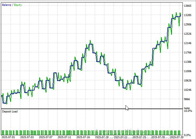
Unfortunately, testing over a period longer than a month is problematic — each month of testing increases the run time by approximately half an hour, even on a new 8-core CPU.

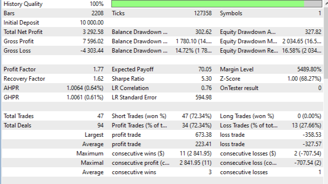
The percentage of profitable trades of 72.3% is significantly higher than the random baseline, which indicates the predictive power of the model. The average winning trade was +223 pips versus the average losing trade of -327 pips, resulting in a favorable profit-to-loss ratio. The maximum series of profits reached 3 trades, the maximum series of losses was limited to 1 trade. Profit Factor 1.77 demonstrates a consistent excess of profits over losses.

Conclusion

PatchTST demonstrates how modern machine learning models can be applied to trading. The patching approach makes the algorithm run faster and allows it to take into account both long-term dependencies and local patterns. The system can adapt to changing market conditions and can be integrated into MetaTrader 5, making it suitable for practical use.

At the same time, the model has limitations. It requires a lot of resources and high-quality historical data. Sharp changes in the market may temporarily reduce the accuracy of forecasts. Like any strategy, it is not immune to "black swan" events and may lose effectiveness over time due to competition and regulatory changes.