Extreme Value Theory in MQL5: Building a Tail-Risk Crash Gauge Beyond Monte Carlo VaR

Introduction

Every risk tool in the average MetaTrader 5 toolbox shares a hidden assumption: that the worst loss worth planning for is roughly the worst loss you have already seen. Average True Range sizes positions from recent volatility. A Monte Carlo resampler shuffles the trades you actually took. Historical Value at Risk reads a percentile straight off your return history. All of them are, in effect, looking backwards at the body of the distribution and quietly hoping the future does not produce anything more extreme than the past.

Markets do not cooperate with that hope. Return distributions in finance are fat-tailed: large moves happen far more often, and reach far further, than a normal distribution predicts. The single worst day in a sample is almost never the worst day the market is capable of, and a method that can only "see" losses as bad as the ones already in its window will systematically understate the size of a rare crash. This is not a subtle academic point. It is the difference between a stop that survives a gap and one that does not.

There is a branch of statistics built specifically for this problem, and it is conspicuously absent from the MQL5 landscape. Extreme Value Theory (EVT) does not model the whole distribution; it models only the tail. The tail's shape is justified by a limit theorem rather than assumed, and the fitted model can extrapolate losses beyond anything present in the sample: a 99.9% loss, a move seen roughly once every three years, a number your history never actually produced.

In this article we build EVT natively in MQL5. We implement the Peaks-Over-Threshold method and fit a Generalized Pareto Distribution to the downside tail of returns using the ALGLIB optimizer, with no external dependencies and no Python bridge. From that engine we build a live crash gauge, an indicator that reports EVT Value at Risk, Expected Shortfall, and a tail-heaviness reading directly on the chart. Finally, we put the gauge to work in a small Expert Advisor that uses the EVT tail estimate to size positions, and we measure what it does in the Strategy Tester.

A note on scope. EVT is a risk-magnitude tool, not a market-timing tool. It tells you how bad a rare loss could be, and whether the tail is currently heavy or light. It does not tell you when a crash will arrive or which direction to trade. Everything in this article is framed accordingly: the gauge measures risk, and the overlay reacts to it by controlling exposure, never by predicting direction.

We will cover:

1. Why normal-assumption risk underestimates the tail
2. Extreme Value Theory: Peaks-Over-Threshold and the GPD
3. Building the engine: the CGPDModel class
4. The live crash gauge: the indicator
5. Putting it to work: an EVT position-sizing overlay
6. Limitations and honest verdict
7. Conclusion

Why normal-assumption risk underestimates the tail

Start with the picture every risk model implicitly draws. If daily returns were normally distributed, then the probability of a move larger than three standard deviations would be about one in 740, and a move beyond five standard deviations would be a once-in-a-few-million-days event, something you would never expect to witness in a trading lifetime. Under that assumption, a stop placed a few standard deviations away is, for all practical purposes, safe.

Real financial returns break this story in two ways at once. They are more peaked in the center, with more days of near-zero returns than the normal curve allows, and they are fatter in the tails, with far more large moves. The five-sigma event that should never happen shows up every few years. The two distributions can have the same mean and the same standard deviation and still disagree violently about exactly the thing risk management cares about: the size of the rare loss.

Fig. 1. The normal model (curve) versus the real fat-tailed returns (histogram); the shaded left tail is the loss it misses.

The shaded gap in Fig. 1 is the entire problem in one image. Any method that estimates risk from the body of the distribution, or that assumes a thin-tailed shape, lives in the white area and is blind to the shaded one. This is why historical Value at Risk feels reassuring right up until it fails: it reports the worst loss it has seen, and the market's job is to eventually produce a worse one.

The conventional responses do not solve this. Resampling the trade history, as a Monte Carlo bootstrap does, can only ever reshuffle losses that already occurred; the method cannot manufacture a larger one that was never in the sample. Scaling stops by recent volatility adapts to the body of the distribution but says nothing about how heavy the tail is. To estimate a loss the sample does not contain, we need a method that extrapolates the tail in a principled way, and that is exactly what Extreme Value Theory provides.

Extreme Value Theory: Peaks-Over-Threshold and the GPD

The central idea of the Peaks-Over-Threshold approach is to stop trying to model the whole return distribution and concentrate entirely on its tail. We choose a high threshold u, discard everything below it, and study only the exceedances: the amounts by which losses cross that threshold. For a loss x above the threshold, the exceedance is the excess y = x - u.

The reason this is more than an arbitrary trick is a limit theorem. The Pickands-Balkema-de Haan theorem states that, for a wide class of underlying distributions, the excesses over a high threshold converge, as the threshold rises, to a single family: the Generalized Pareto Distribution (GPD). So while we do not know and do not assume the shape of the whole return distribution, we have a theoretical justification for the shape of its tail. The tail is described by the GPD survival function:

P(X - u > y | X > u) = (1 + xi * y / sigma)^(-1/xi)

This tends to exp(-y / sigma) as xi approaches 0.

The GPD has just two parameters, and both carry direct meaning for a trader:

• The shape parameter xi. This is the tail-heaviness dial. When xi is greater than zero the tail is heavy and Pareto-like, the regime of fat tails and crashes; the larger xi, the heavier the tail. When xi is near zero the tail decays exponentially. A rising xi is the single most direct statement that tail risk is building.
• The scale parameter sigma. A strictly positive spread parameter that sets the size of typical exceedances above the threshold.

Fig. 2. Peaks-Over-Threshold: set a threshold u, collect the exceedances above it, and fit a GPD to those excesses.

Once the two parameters are fitted, the payoff is that the tail becomes a formula we can evaluate at any confidence level, including levels beyond the sample. The Value at Risk at confidence p is the loss we do not expect to exceed with probability p:

VaR_p = u + (sigma / xi) * [ (n / Nu * (1 - p))^(-xi) - 1 ]

Here Nu/n is the exceedance rate, the fraction of observations that lie above the threshold.

Value at Risk answers "how bad, at the edge?" but says nothing about what happens once you are past that edge. Expected Shortfall, also called Conditional VaR, fills that gap: it is the average loss given that the VaR level has been breached, the expected size of the bad day once you are already having one. For the GPD it has a clean closed form:

ES_p = VaR_p / (1 - xi) + (sigma - xi * u) / (1 - xi)

This is valid for xi < 1.

The condition xi < 1 is not a technicality to gloss over: when xi reaches one, the theoretical mean of the tail becomes infinite and Expected Shortfall is undefined. That is the model telling you the tail is so heavy that the notion of an "average loss beyond VaR" stops making sense, and our implementation respects that boundary rather than returning a meaningless number.

Three quantities, then, summarize the entire tail: VaR (how bad at the edge), ES (how bad beyond it), and xi (how heavy the tail is right now). The rest of this article turns these formulas into working MQL5.

Building the engine: the CGPDModel class

All of the EVT mathematics lives in a single, reusable header, GPDModel.mqh, so that both the indicator and the Expert Advisor can share one source of truth. The engine has one job: take an array of losses, fit the GPD tail, and expose VaR, Expected Shortfall, and the fitted parameters. Before any of that, it declares how it reports its own trustworthiness, because an EVT estimate built on too little tail data is worse than useless, it is confidently wrong.

//--- model status / data-sufficiency flag
enum ENUM_GPD_STATUS
  {
   GPD_OK,                 // fit succeeded and is usable
   GPD_NOT_FITTED,         // Fit() not called yet
   GPD_TOO_FEW_EXCEEDANCES,// not enough tail data for a trustworthy fit
   GPD_FIT_FAILED,         // optimizer did not converge to a valid solution
   GPD_BAD_INPUT           // empty / degenerate input
  };

//--- minimum exceedances below which a GPD fit is not trustworthy.
//--- EVT literature treats ~30-50 tail points as a practical floor.
#define GPD_MIN_EXCEEDANCES 30

The status enum is the engine's honesty mechanism. Any fit that does not earn GPD_OK causes the risk metrics to return zero rather than a fabricated figure, and the reason is reported back to the caller. The GPD_MIN_EXCEEDANCES floor of 30 reflects standard EVT practice: below roughly thirty tail points, the two-parameter fit is too unstable to believe. This single constant is what later lets the gauge say "insufficient data" out loud instead of printing a confident lie.

The likelihood objective

The two GPD parameters are estimated by maximum likelihood, which means we minimize the negative log-likelihood of the exceedances. ALGLIB's optimizers call a user-supplied objective object, so we implement one by subclassing CNDimensional_Func. It holds a copy of the exceedances and, given a candidate parameter vector, returns the negative log-likelihood.

//+------------------------------------------------------------------+
//| GPD negative log-likelihood.                                     |
//|  For xi ~ 0 we use the exponential limit to stay numerically     |
//|  stable. Invalid parameter regions return a large penalty so the |
//|  optimizer is repelled rather than producing NaNs.               |
//+------------------------------------------------------------------+
void CGPDNegLogLik::Func(double &x[],double &func,CObject &obj)
  {
   double xi    = x[0];
   double sigma = x[1];
   const double BIG = 1.0e15;

   if(sigma<=0.0)
     {
      func=BIG;
      return;
     }

   double nll=0.0;
   for(int i=0;i<m_n;i++)
     {
      double y=m_excess[i];
      double z=y/sigma;
      if(MathAbs(xi)<1.0e-8)
        {
         //--- exponential limit: log f = -log(sigma) - y/sigma
         nll += MathLog(sigma) + z;
        }
      else
        {
         double t=1.0+xi*z;
         if(t<=0.0)
           {
            //--- excess outside the GPD support for this xi: reject
            func=BIG;
            return;
           }
         //--- log f = -log(sigma) - (1 + 1/xi) * log(1 + xi*z)
         nll += MathLog(sigma) + (1.0+1.0/xi)*MathLog(t);
        }
     }
   func=nll;
  }

Two defensive details make this robust. When xi is numerically indistinguishable from zero, the general formula would divide by it, so we switch to the exponential limit of the GPD. And when a candidate xi would place an observed excess outside the distribution's support, we return a large penalty value, which repels the optimizer from that region instead of letting it produce a not-a-number that would poison the search.

The fit pipeline

The public Fit method orchestrates the whole process: sort the losses, locate the threshold as a quantile of them, peel off the exceedances, check there are enough of them, and only then run the optimizer.

//--- sort losses ascending to locate the threshold quantile
   double sorted[];
   ArrayResize(sorted,count);
   for(int i=0;i<count;i++)
      sorted[i]=losses[i];
   ArraySort(sorted);

   m_u=Quantile(sorted,count,m_threshold_q);

//--- collect excesses over u (strictly positive)
   double excess[];
   int k=0;
   ArrayResize(excess,count);
   for(int i=0;i<count;i++)
     {
      double e=losses[i]-m_u;
      if(e>0.0)
         excess[k++]=e;
     }
   ArrayResize(excess,k);
   m_n_exceed=k;

   if(k<GPD_MIN_EXCEEDANCES)
     {
      m_status=GPD_TOO_FEW_EXCEEDANCES;
      return false;
     }

By default the threshold is the 95th percentile of the loss sample, so the top five percent of losses become the exceedances we model. This is where the data-sufficiency check bites: at a 95% threshold, a window of n bars yields only about 5% of n exceedances, so the window has to be large enough to clear the floor of thirty. We will see this constraint surface concretely when we run the indicator.

The maximum-likelihood fit

With the exceedances in hand, RunMLE drives the ALGLIB optimizer. We use MinBLEIC, the bound-constrained optimizer, in its finite-difference variant so that we do not have to derive and hand-code the likelihood gradient; ALGLIB differentiates the objective numerically.

//--- box constraints: xi in [-0.5, 1.0], sigma in (eps, +inf)
   double bndl[];
   ArrayResize(bndl,2);
   double bndu[];
   ArrayResize(bndu,2);
   bndl[0]=-0.5;
   bndu[0]=1.0;
   bndl[1]=1.0e-12;
   bndu[1]=CInfOrNaN::PositiveInfinity();

   CMinBLEICStateShell  state;
   CMinBLEICReportShell rep;
   CGPDNegLogLik        objective;
   CNDimensional_Rep    repcb;
   CObject              dummy;

   objective.SetData(excess,n);

//--- finite-difference variant: we supply only the function value.
   double diffstep=1.0e-6;
   CAlglib::MinBLEICCreateF(2,x,diffstep,state);
   CAlglib::MinBLEICSetBC(state,bndl,bndu);
//--- inner stop: epsg, epsf, epsx ; outer stop: epsx, epsi
   CAlglib::MinBLEICSetInnerCond(state,0.0,0.0,1.0e-8);
   CAlglib::MinBLEICSetOuterCond(state,1.0e-8,1.0e-8);
   CAlglib::MinBLEICOptimize(state,objective,repcb,false,dummy);

The box constraints encode what a valid GPD looks like. The scale sigma is held strictly positive by a lower bound just above zero with no upper limit. The shape xi is confined to the range from minus one-half to one, which spans every tail regime we care about while keeping the search away from degenerate corners; in particular the upper bound of one is the same boundary beyond which Expected Shortfall ceases to exist.

Seeding the optimizer

One detail in RunMLE deserves more than a passing mention, because it is the difference between a fit that converges and one that wanders. We use the finite-difference optimizer, which does not see the likelihood's analytic gradient; it probes the objective numerically. Such a search is only as good as its starting point, and starting from an arbitrary guess invites slow convergence or a local trap. So before the optimizer runs, we hand it a closed-form estimate of the two parameters derived from the first two moments of the exceedances, the classic method-of-moments seed for the GPD:

//--- starting point: method-of-moments seed for robustness
   double mean=0.0;
   for(int i=0;i<n;i++)
      mean+=excess[i];
   mean/=n;
   double var=0.0;
   for(int i=0;i<n;i++)
      var+=(excess[i]-mean)*(excess[i]-mean);
   var/=MathMax(1,n-1);

//--- MoM: xi0 = 0.5*(1 - mean^2/var), sigma0 = 0.5*mean*(mean^2/var + 1)
   double ratio=(var>0.0)?(mean*mean/var):1.0;
   double xi0   = 0.5*(1.0-ratio);
   double sig0  = 0.5*mean*(ratio+1.0);
   if(!MathIsValidNumber(xi0)  || xi0<-0.4 || xi0>0.9)
      xi0=0.1;
   if(!MathIsValidNumber(sig0) || sig0<=0.0)
      sig0=MathMax(mean,1.0e-8);

The two formulas in the comment come from equating the GPD's theoretical mean and variance to the sample mean and variance of the exceedances and solving for the parameters. That gives a seed that is usually already close to the answer, so the optimizer mostly has to polish it rather than discover it. The two guard clauses matter as much as the formulas: a degenerate sample can make the method-of-moments estimate produce a meaningless or out-of-range value, so an xi0 outside a sane band falls back to a neutral 0.1 and a non-positive sigma0 falls back to the sample mean. Even the seed is not trusted blindly, which is in keeping with the rest of the engine.

From parameters to risk numbers

Once xi and sigma are fitted, the VaR and Expected Shortfall methods are direct transcriptions of the formulas from the previous section, each with the exponential limit handled for the near-zero-xi case.

//+------------------------------------------------------------------+
//| GPD-POT Value at Risk at confidence p (e.g. 0.99).               |
//|  VaR_p = u + (sigma/xi)*[ ( n/Nu * (1-p) )^(-xi) - 1 ]           |
//|  with the exponential limit as xi -> 0.                          |
//|  Nu/n is the exceedance rate = m_n_exceed / m_n_total.           |
//+------------------------------------------------------------------+
double CGPDModel::VaR(double p) const
  {
   if(m_status!=GPD_OK)
      return 0.0;
   if(p<=0.0 || p>=1.0)
      return 0.0;

   double rate=(double)m_n_exceed/(double)m_n_total; // Nu/n
   if(rate<=0.0)
      return 0.0;

   double frac=(1.0-p)/rate;       // = n/Nu * (1-p)
   if(frac<=0.0)
      return m_u;

   if(MathAbs(m_xi)<1.0e-8)
      return m_u - m_sigma*MathLog(frac);            // exponential limit
   return m_u + (m_sigma/m_xi)*(MathPow(frac,-m_xi)-1.0);
  }

Notice the very first line of the method. If the model is not in the GPD_OK state, VaR returns zero, and Expected Shortfall does the same. The honesty rule is enforced at the point of use, not merely advertised: there is no path by which an unreliable fit can hand back a plausible-looking risk number. With the engine complete and self-contained, we can now give it a face.

The live crash gauge: the indicator

The indicator, EVTCrashGauge.mq5, turns the engine into something you watch. On every new bar it takes a rolling window of recent closes, converts them into a downside-loss series, fits the GPD, and reports the result both as an on-chart panel and as a plotted Value-at-Risk line in a sub-window. Its inputs are deliberately few.

//--- inputs
input int    Lookback        = 800;    // rolling window (bars) for the fit
input double ThresholdQuant  = 0.95;   // POT threshold quantile
input double Confidence      = 0.99;   // VaR/ES confidence
input int    RefitEvery      = 1;      // refit every N new bars
input bool   ShowPanel       = true;   // draw the on-chart text panel

The downside-loss series is the conceptual bridge between price and the engine. For each pair of consecutive closes we take the log return, and we keep only the magnitude of the down moves, mapping every up move to zero. This is the one-sided "crash" framing: we are modeling the tail of losses, so gains contribute nothing to it.

//+------------------------------------------------------------------+
//| Build the downside-loss series from a window of closes ending at |
//| bar index 'end' (older->newer) and fit the GPD.                  |
//|  loss_i = max(0, -logreturn_i) = magnitude of a down move.       |
//+------------------------------------------------------------------+
bool FitWindow(const double &close[],int end,int total)
  {
   int start=end-Lookback;          // need Lookback returns
   if(start<1)
      return false;

   double losses[];
   int k=0;
   ArrayResize(losses,end-start+1);    // loop runs (end-start+1) times
   for(int i=start;i<=end;i++)
     {
      if(i<1 || i>=total)
         continue;
      if(close[i-1]<=0.0 || close[i]<=0.0)
         continue;
      double r=MathLog(close[i]/close[i-1]);   // log return
      double loss=(r<0.0)?-r:0.0;              // downside magnitude
      losses[k++]=loss;
     }
   if(k<Lookback/2)
      return false;           // window too sparse
   ArrayResize(losses,k);

   return g_model.Fit(losses,k);
  }

How the gauge updates across bars

A GPD fit is an optimization, not a lookup, so refitting on every historical bar of a long chart would be wasteful. The indicator handles this in OnCalculate with a small cadence rule: the most recent bar is always refitted so the live reading is current, while older bars are refitted only every RefitEvery bars, governed by a countdown in g_bars_since_fit. The result that a fit produces is then written into the plotted VaR buffer for that bar.

   for(int bar=start;bar<rates_total;bar++)
     {
      bool do_fit=(bar==rates_total-1) || (g_bars_since_fit<=0);
      if(do_fit)
        {
         if(FitWindow(close,bar,rates_total))
           {
            g_status =g_model.Status();
            g_xi     =g_model.Xi();
            g_exceed =g_model.ExceedanceCount();
            g_var    =g_model.VaR(Confidence);
            g_es     =g_model.ExpectedShortfall(Confidence);
           }
         else
            g_status=g_model.Status();
         g_bars_since_fit=RefitEvery;
        }
      else
         g_bars_since_fit--;

      VaRBuffer[bar]=(g_status==GPD_OK)?g_var:0.0;
     }

With RefitEvery at its default of 1, every bar is refitted and the plotted line is fully resolved; raising it trades some historical resolution for speed on very long charts, while the current bar always stays exact. Whenever a fit does not earn GPD_OK, the buffer is set to zero for that bar rather than carrying a stale value forward, so the plotted line is blank exactly where the model declined to commit to a number.

The panel reads off the fitted model and color-codes the tail. When the fit is reliable it shows the VaR and Expected Shortfall at the chosen confidence as percentages, and the shape xi with a traffic-light color: green for a light tail, gold for moderately heavy, red for the heavy-tailed regime where crashes cluster. When the fit is not reliable, the panel says so plainly.

void UpdatePanel()
  {
   if(g_status!=GPD_OK)
     {
      ObjectSetString(0,g_prefix+"var",OBJPROP_TEXT,"VaR : --");
      ObjectSetString(0,g_prefix+"es",OBJPROP_TEXT,"ES  : --");
      ObjectSetString(0,g_prefix+"xi",OBJPROP_TEXT,"xi  : --");
      ObjectSetInteger(0,g_prefix+"xi",OBJPROP_COLOR,clrGray);
      ObjectSetString(0,g_prefix+"status",OBJPROP_TEXT,"status: "+g_model.StatusText());
      ObjectSetInteger(0,g_prefix+"status",OBJPROP_COLOR,clrSilver);
      return;
     }

The traffic-light itself is a tiny helper, and it is worth being explicit about where the cutoffs sit rather than leaving the colors vague:

//+------------------------------------------------------------------+
//| Map xi to a tail-heaviness color (calm -> elevated -> extreme).  |
//+------------------------------------------------------------------+
color XiColor(double xi)
  {
   if(xi<0.10)
      return clrLimeGreen;     // light tail, calm
   if(xi<0.30)
      return clrGold;          // moderately heavy
   return clrOrangeRed;                 // heavy tail, extreme
  }

The boundaries are deliberately rounded rather than precise: a shape below 0.10 is close enough to the exponential, thin-tailed regime to read as calm, the band up to 0.30 is the everyday moderately-heavy zone most liquid instruments live in, and anything above 0.30 is the territory where losses compound and crashes cluster. These are reading aids, not hard statistical thresholds, and a trader who wanted a stricter or looser dashboard could shift them freely. What matters is that the same xi that drives the math also drives the color, so the panel cannot show green while the formula is quietly computing a fat-tailed VaR.

This is where the data-sufficiency floor becomes concrete. With the lookback set to 500 bars on a 95% threshold, the gauge gets only about twenty-five exceedances, below the floor of thirty, so the panel refuses to fit, reporting insufficient tail data (25/30 exceedances) instead of a number. Raising the lookback to 800 bars clears the floor and the gauge fits cleanly. That is not a bug to work around; it is the model declining to guess, which is precisely the behavior we want from a tool whose entire purpose is to be honest about rare events.

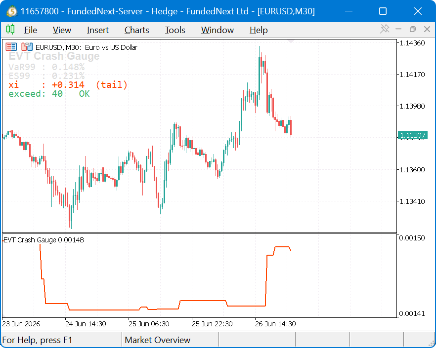
Fig. 3. The EVT Crash Gauge on a chart: the panel reports VaR, Expected Shortfall, and the color-coded tail shape xi, while the sub-window plots the EVT VaR over time so the tail can be seen tightening and loosening.

Read as a gauge rather than a signal, the value of the plotted line is that you can watch the tail breathe. When the VaR line lifts and xi turns from green toward red, the market's downside tail is fattening, and the appropriate response is defensive: smaller positions, wider mental stops, more caution, not a directional bet. Making that response automatic is the subject of the next section.

Putting it to work: an EVT position-sizing overlay

To show the gauge doing something rather than merely displaying something, we wrap it in a minimal Expert Advisor, EVTRiskOverlay.mq5. This EA is not about its entry logic, which is a deliberately trivial moving-average cross; it is about its overlay. Before each trade, the overlay consults the EVT tail estimate and sizes the position so that the estimated tail loss stays within a fixed fraction of equity. A single master switch lets us run the identical strategy with the overlay off or on.

//--- EVT overlay
input bool   UseEVT          = true;   // master toggle (off = baseline)
input int    Lookback        = 800;    // window for the GPD fit (>=~800 for 30+ tail pts at q=0.95)
input double ThresholdQuant  = 0.95;   // POT threshold quantile
input double Confidence      = 0.99;   // VaR confidence
input double EquityBudgetPct = 2.0;    // max tolerated EVT tail loss (% equity)
input bool   BlockOverScale  = false;  // true: block trade; false: halve lot

The EA first asks the engine for the current tail estimate. The EVTValueAtRisk helper rebuilds the downside-loss window from recent closed bars, fits the model, and returns the EVT VaR as a fractional return, or a negative sentinel if the fit was not reliable. That sentinel matters: an unreliable tail estimate must never be silently treated as "low risk".

The sizing itself is the heart of the overlay, but it depends on one piece of plumbing that does the unit conversion. EVT VaR is a per-bar fractional loss, a pure number like 0.018 meaning a 1.8% adverse move; an equity budget, on the other hand, is an amount of account currency. To compare the two we need to know what that fractional move costs in money for one lot of the instrument we are trading. That is the job of LossPerLot:

//+------------------------------------------------------------------+
//| Money value of a 1-lot position if price moves by 'ret' fraction.|
//|  Uses the symbol's tick value/size so it works across FX,        |
//|  indices, metals, etc. Returns loss in account currency for one  |
//|  lot given a fractional adverse move.                            |
//+------------------------------------------------------------------+
double LossPerLot(double ret)
  {
   double price=SymbolInfoDouble(_Symbol,SYMBOL_BID);
   double tickVal=SymbolInfoDouble(_Symbol,SYMBOL_TRADE_TICK_VALUE);
   double tickSz =SymbolInfoDouble(_Symbol,SYMBOL_TRADE_TICK_SIZE);
   if(tickSz<=0.0 || price<=0.0)
      return 0.0;
   double priceMove=ret*price;                 // adverse move in price terms
   return (priceMove/tickSz)*tickVal;          // currency loss for 1.0 lot
  }

The conversion is two steps. First the fractional return is turned into an absolute price move by multiplying by the current price, so a 1.8% move on a price of 1.0850 becomes about 0.0195 in quote terms. Then that price move is expressed in ticks and multiplied by the value of one tick, which is what SYMBOL_TRADE_TICK_VALUE and SYMBOL_TRADE_TICK_SIZE report for the symbol. Because those two properties already encode each instrument's contract size and quote currency, the same function returns a correct per-lot loss whether the symbol is a forex pair, a stock index, or a metal, with no special-casing in the overlay above it. From there, sizing the position is a single division.

//+------------------------------------------------------------------+
//| EVT position sizer (the overlay).                                |
//|  Translate EVT VaR into the position's tail loss as a fraction   |
//|  of equity and size the lot so estimated tail loss stays within  |
//|  the equity budget:                                              |
//|     max_lot = (budget * equity) / (LossPerLot(VaR))              |
//|  Final lot = min(base lot, max_lot). Calm tail -> full base lot; |
//|  fat tail -> automatically scaled down. Returns 0.0 = no trade.  |
//+------------------------------------------------------------------+
double OverlayLot()
  {
   double lot=BaseLot;
   if(!UseEVT)
      return lot;

   double var=EVTValueAtRisk();
   if(var<0.0)                  // unreliable fit -> be conservative, skip
      return 0.0;

   double equity=AccountInfoDouble(ACCOUNT_EQUITY);
   double budget=EquityBudgetPct/100.0;     // e.g. 0.02
   double lossPerLot=LossPerLot(var);          // currency tail loss / lot
   if(lossPerLot<=0.0)
      return lot;                              // can't size -> fall back to base

   double maxLot=(budget*equity)/lossPerLot;   // lot meeting the budget exactly

   if(BlockOverScale && maxLot<lot)
      return 0.0;                              // strict mode: veto oversized trades
   return MathMin(lot,maxLot);                 // sizer mode: cap at budget
  }

The logic reads cleanly once the scaling is right. We compute the largest lot whose estimated tail loss equals the equity budget, then trade the smaller of that and the base lot. When the tail is calm, the budget-implied lot is large and we trade the full base size; when the tail is fat, the budget-implied lot shrinks and the position is automatically scaled down. The behavior is continuous: the overlay does not wait for a binary alarm, it leans on the throttle in proportion to how heavy the tail is right now.

Two branches in that function are worth drawing out, because they are where the overlay's risk posture is decided. The first is the very top: if EVTValueAtRisk returns its negative sentinel, meaning the fit was not reliable, OverlayLot returns zero and the trade is skipped entirely. This is the deliberate choice to treat "we do not know the tail" as a reason for caution rather than a green light; an unreliable estimate is never quietly read as low risk. The second is the BlockOverScale switch at the bottom, which selects between the overlay's two modes. In the default sizer mode it returns min(base lot, max lot), capping the position at the budget but still taking the trade. In strict mode, when BlockOverScale is true, it instead returns zero whenever the budget-implied lot is smaller than the base lot, vetoing any trade the tail says is too large to take at full size. Sizer mode throttles; strict mode refuses. The backtest below uses sizer mode, which is why, as we will see, it changes the size of every trade without removing any.

The comparison

We run the EA twice over the same year-plus of history on the same symbol and timeframe, changing only UseEVT. With the overlay off we have a pure baseline; with it on, the EVT sizer is the only thing that differs. The results are summarized below.

Metric	Baseline (EVT off)	EVT overlay on
Total net profit	-333.60	-223.99
Profit factor	0.87	0.90
Expected payoff	-3.44	-2.31
Recovery factor	-0.45	-0.40
Sharpe ratio	-0.88	-0.66
Balance drawdown maximal	715.70	540.90
Equity drawdown maximal	733.50	556.75
Largest loss trade	-59.60	-52.00
Total trades	97	97

The single most important row is the last one. Both runs took exactly 97 trades. The overlay vetoed nothing; it took every entry the baseline took. The only thing it changed was the size of those positions, scaling them down when the tail was heavy. With the entries held constant as a control, every difference in the table is attributable to position sizing alone, which is as clean a demonstration of the mechanism as a backtest can offer.

And the effect is exactly what an EVT overlay is supposed to produce. Maximum equity drawdown fell by about 24%, from 733.50 to 556.75, with the same improvement in balance drawdown and a smaller worst single loss. The risk-adjusted metrics, Sharpe and recovery factor, both improved, and net loss shrank as a side effect of carrying less exposure during dangerous periods.

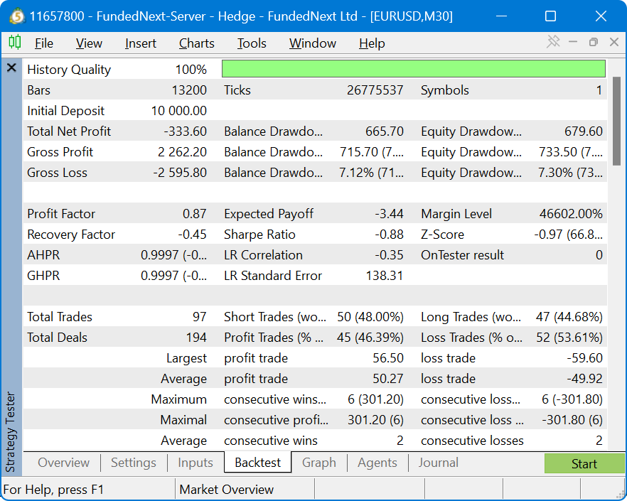
Fig. 4. Baseline equity curve with the overlay off (UseEVT = false).

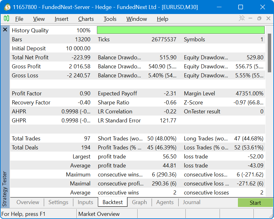
Fig. 5. Equity curve with the EVT overlay on. The same 97 entries are taken, but positions are scaled down in heavy-tailed periods, producing a shallower drawdown.

NOTE: Both versions of the strategy lose money: the moving-average cross is a placeholder, not an edge, and EVT does not turn a losing system into a winning one. The claim being made, and the only claim the data supports, is narrow and real: holding the entries fixed, EVT-based sizing cut maximum drawdown by roughly a quarter. EVT controls the severity of tail losses; it does not generate returns.

Limitations and honest verdict

EVT earns its place in a risk toolkit, but it is a specialized instrument, and using it well means knowing where it does and does not apply.

• It is hungry for tail data. A two-parameter tail fit needs a meaningful number of exceedances, which is why the engine enforces a floor and why a 500-bar window failed where 800 succeeded. On a thinly traded symbol or a very short window, the right answer from the model is "insufficient data", and the design honors that rather than inventing a number.
• It is sensitive to the threshold. The choice of the 95th percentile is a standard default, but the fitted shape and scale do shift with the threshold. A serious deployment would examine that sensitivity rather than trusting a single setting, and the threshold quantile is exposed as an input precisely so it can be studied.
• It measures magnitude, not timing. This bears repeating because it is the most common way EVT is misused. The gauge tells you how heavy the tail is and how large a rare loss could be; it does not predict the next crash or imply a direction. Treating a rising xi as a "go short" signal is a misreading of the tool.
• The tail can stop being well-defined. When the fitted xi approaches one, the mean of the tail diverges and Expected Shortfall becomes meaningless. The engine returns zero in that regime rather than a fabricated figure, which is itself information: the tail is too heavy for an average-beyond-VaR to exist.

Within those limits, the verdict is positive. EVT fills a real and previously empty slot in the MQL5 risk landscape: a principled way to estimate losses the sample has not yet produced, and a live reading of how fat the downside tail currently is. As the overlay showed, wiring that estimate into position sizing reduces drawdown materially for an unchanged set of entries, which is exactly the job a tail-risk model should do.

Conclusion

We set out to bring Extreme Value Theory, the statistics of rare events, into MetaTrader 5, and to do it honestly. Along the way we built a complete, self-contained tail-risk stack.

• A reusable engine. The CGPDModel class fits a Generalized Pareto Distribution to the downside tail by maximum likelihood using ALGLIB, with no external dependencies, and exposes VaR, Expected Shortfall, and the tail-shape xi, while refusing to report numbers it cannot stand behind.
• A live crash gauge. The indicator turns that engine into an on-chart panel and a VaR line, color-coding tail heaviness and saying "insufficient data" out loud when the tail sample is too thin to trust.
• A working overlay. The Expert Advisor converts the EVT tail estimate into position sizing and, in a year-plus backtest, cut maximum drawdown by roughly 24% while taking the identical set of trades.

The throughline is that EVT is a measurement, and the right way to act on a measurement of risk is to control exposure, not to predict direction. Used that way, it is a genuinely useful addition to a trader's toolkit, and one the MQL5 community has not had until now. The natural extensions, from threshold-stability diagnostics to two-sided tails and intraday timeframes, are left as directions for further work.

The programs presented in this article are intended for educational purposes only. Trading carries a high level of risk, and past performance, including backtested results, is not indicative of future results. Always test thoroughly on a demo account before risking real capital.

Getting the Source Code via MQL5 Algo Forge

All source files are attached to this article below, but the full repository is also available on MQL5 Algo Forge, the community's Git-based platform for sharing and collaborating on trading projects.

File name	Description
MQL5\Include\EVT\GPDModel.mqh	Extreme Value Theory tail-risk engine: Peaks-Over-Threshold GPD fit via ALGLIB, with VaR and Expected Shortfall
MQL5\Indicators\EVT\EVTCrashGauge.mq5	The crash-gauge indicator: on-chart VaR, Expected Shortfall, and tail-shape panel plus a plotted EVT VaR line
MQL5\Experts\EVT\EVTRiskOverlay.mq5	Minimal Expert Advisor demonstrating EVT-based position sizing, with a toggle for the before/after comparison