Measuring What Matters (Part 2): Building the Covariance Matrix: Eigenvalue Decomposition and Risk Factor Analysis in MQL5

Introduction

In Part 1 of this series, we built PortfolioRiskAnalyzer.mq5 — a script that exposed a gap most multi-symbol traders never see. By computing the full covariance matrix using the native OpenBLAS .Cov() method and then performing the true portfolio variance calculation as a proper matrix multiplication — wᵀ Σ w — we showed that the true risk of holding EURUSD, GBPUSD, and XAUUSD simultaneously can be materially higher than what naive single-instrument volatility suggests.

What Part 1 produced was a single number: the hidden risk gap. That number was concrete, readable, and immediately useful. It compressed the covariance information into one output. The 3 × 3 matrix was computed by all_returns.Cov() and used for wᵀ Σ w, but it was never stored or printed. The reader could see the gap but could not yet see inside the matrix that produced it.

Part 2 changes that. We introduce the CCovarianceMatrix class—an object-oriented wrapper around OpenBLAS .Cov(). It stores the covariance matrix, verifies symmetry, and prints a labeled grid. It then calls the native MQL5 .Eig() method to obtain eigenvalues and eigenvectors, showing which factors drive risk and how each symbol loads on them.

The practical project for Part 2 is CovarianceMatrixPrinter.mq5. It builds a 3 x 3 covariance matrix, verifies symmetry, prints a labeled grid, and generates a risk-factor report that exposes the portfolio's factor structure.

What Part 1 Built — and What It Could Not Show

To understand what Part 2 adds, we need to be precise about what Part 1 actually did. In PortfolioRiskAnalyzer.mq5, the covariance matrix was computed in three lines:

//---From PortfolioRiskAnalyzer.mq5 — Part 1
  matrix all_returns;
  all_returns.Init(3, LookbackBars);
  all_returns.Row(returns1, 0);
  all_returns.Row(returns2, 1);
  all_returns.Row(returns3, 2);

  matrix cov_matrix = all_returns.Cov();

Assets were laid out as rows, observations as columns — the layout that MQL5's .Cov() method requires to return a correct [Asset x Asset] covariance matrix. The resulting cov_matrix was a 3 x 3 matrix where each entry [i][j] held the covariance between asset i and asset j. This is the correct, OpenBLAS-accelerated approach.

But immediately after building the matrix, Part 1 used it for one purpose only:

//---From PortfolioRiskAnalyzer.mq5 — Part 1
  vector intermediate = cov_matrix.MatMul(w);   // Step A: Cov * w
  double true_variance = w.Dot(intermediate);   // Step B: w^T * (Cov * w)

The matrix was multiplied by the weight vector to produce one scalar — true_variance. After that calculation, the matrix was no longer referenced. Its internal structure — which symbols are correlated with which, how strongly, and in what directions — was never exposed to the reader.

This is the structural limitation Part 2 resolves. By encapsulating the matrix inside a class, we can store it persistently, print every cell with its symbol labels, verify its symmetry, and decompose it into eigenvalues and eigenvectors. Each of those steps reveals something the single gap number from Part 1 could not show.

The Architecture Upgrade: Why a Class

This script's OnStart() must build, store, verify, print, and decompose the matrix. In future parts we will pass it to indicators and EAs for continuous use. A flat, linear script structure does not scale well to that many responsibilities.

A class is the right structure for this because it groups three things that belong together: the matrix data, the symbol names that label its rows and columns, and the methods that operate on it. Once the CCovarianceMatrix object is instantiated and built, every operation — printing, symmetry checking, eigendecomposition — is a method call on that object. OnStart() stays clean. The class itself becomes a reusable component that Parts 3 through 10 will import directly.

Setting Up the Script: Properties and Inputs

Open MetaEditor and create a new Script file named CovarianceMatrixPrinter.mq5. The property declarations and inputs are straightforward — we don't need portfolio weight inputs because this script's purpose is to examine the matrix structure, not compute a weighted risk number:

#property copyright   "Measuring What Matters Series — Part 2"
#property link        ""
#property version     "1.01"
#property script_show_inputs

input string          Symbol1       = "EURUSD";
input string          Symbol2       = "GBPUSD";
input string          Symbol3       = "XAUUSD";
input ENUM_TIMEFRAMES TF            = PERIOD_H1;
input int             LookbackBars  = 100;

This script requires only the three symbols, the timeframe, and the lookback period. Portfolio weights are intentionally omitted because the objective is no longer to compute a weighted portfolio variance. Instead, the script analyzes the covariance matrix itself through structural inspection and eigenvalue decomposition. These operations depend only on the relationships between the instruments, not on how capital is allocated among them.

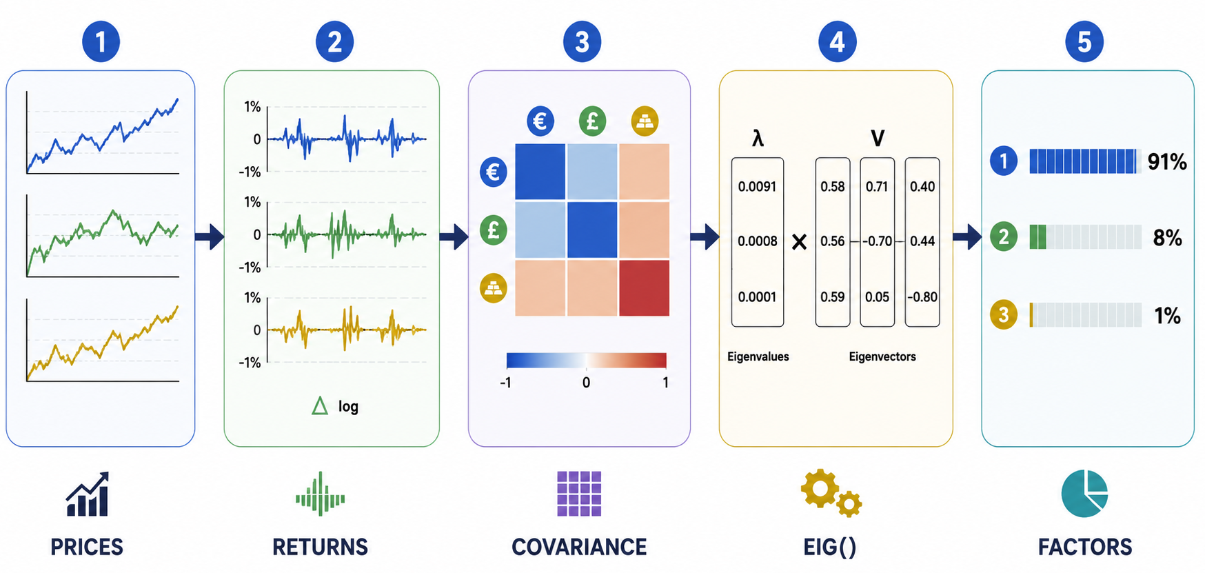
The ComputeLogReturns Function

The first function in the script is ComputeLogReturns. It collects closing prices, converts them into logarithmic returns, and prepares the return vectors used throughout the covariance analysis. Rather than leaving this workflow embedded in the script logic, the surrounding matrix operations are now organized inside an object-oriented MQL5 class, making the overall design easier to reuse and extend.

//+------------------------------------------------------------------+
//| Helper: Compute log returns                                      |
//+------------------------------------------------------------------+
bool ComputeLogReturns(const string symbol,
                       ENUM_TIMEFRAMES tf,
                       int bars,
                       vector &log_returns)
  {
   vector prices;
   if(!prices.CopyRates(symbol, tf, COPY_RATES_CLOSE, 0, bars + 1))
     {
      PrintFormat("ERROR: Could not copy rates for %s. Error: %d",
                  symbol, GetLastError());
      return false;
     }

   log_returns.Init(bars);

   for(int i = 0; i < bars; i++)
     {
      if(prices[i] <= 0.0 || prices[i + 1] <= 0.0)
        {
         log_returns[i] = 0.0;
         continue;
        }
      log_returns[i] = MathLog(prices[i] / prices[i + 1]);
     }

   return true;
  }

Every design decision here is deliberate: bars + 1 prices are read to produce N returns, the MathLog(prices[i] / prices[i+1]) formula computes the logarithmic return, a zero-price guard prevents invalid values, and the function returns early on failure. This function is the permanent data foundation of this series and will appear unchanged in every subsequent part.

The PrintDivider helper is also included:

//+------------------------------------------------------------------+
//| Helper: Print a formatted divider line                           |
//+------------------------------------------------------------------+
void PrintDivider(string ch = "-", int len = 55)
  {
   string line = "";
   for(int i = 0; i < len; i++) line += ch;
   Print(line);
  }

Building the CCovarianceMatrix Class

The class declaration begins with three private members:

//+------------------------------------------------------------------+
//| CLASS: CCovarianceMatrix                                         |
//| Encapsulates the full covariance matrix workflow:                |
//|   - Stores symbol names and scales matrix dimensions dynamically |
//|   - Builds the covariance matrix natively using OpenBLAS         |
//|   - Verifies structural matrix symmetry                          |
//|   - Provides eigenvalue decomposition via native .Eig()          |
//|   - Prints formatted matrix grids and risk factor loading spectra|
//+------------------------------------------------------------------+
class CCovarianceMatrix
  {
private:
   int               m_size;
   string            m_symbols[];
   matrix            m_cov;

m_size stores the number of symbols — the dimension of the square matrix. m_symbols[] is a dynamic string array holding the symbol names, which are used to label the rows and columns of the printed grid. m_cov is the native MQL5 matrix object that will hold all covariance values once Build() is called.

The m_ prefix on all three members is a naming convention that makes it immediately clear inside any method whether a variable is a member of the class or a local variable. This is a habit worth adopting in any MQL5 project that uses classes.

The Constructor

//--- Constructor
                     CCovarianceMatrix(const string &symbols[], int size)
     {
      m_size = size;
      ArrayResize(m_symbols, m_size);
      for(int i = 0; i < m_size; i++)
         m_symbols[i] = symbols[i];
      m_cov.Init(m_size, m_size);
     }

The constructor takes a string array of symbol names and an integer size. It copies the symbol names into m_symbols— the ArrayResize before the copy loop is required in MQL5 before writing to a dynamic array. It then calls m_cov.Init(m_size, m_size) to allocate the matrix as an m_size by m_size grid of zeros, ready to be filled by Build().

For our three-symbol case this produces a 3 x 3 matrix of zeros. The class is written to handle any size — passing size = 5 with five symbol names produces a 5 x 5 matrix with no structural change to the code.

The Build Method: OpenBLAS at the Core

The Build method is where the actual covariance computation happens:

//--- Build the matrix from return vectors via OpenBLAS structures
   bool              Build(const vector &returns[], int n_vectors)
     {
      if(n_vectors != m_size || n_vectors < 1)
        {
         Print("ERROR: Number of return vectors must match matrix size.");
         return false;
        }

//--- Collect number of columns/observations from the first asset vector
      ulong columns = returns[0].Size();
      matrix all_returns;
      all_returns.Init(m_size, columns);

//--- Systematically populate rows (Assets as Rows, Observations as Columns)
      for(int i = 0; i < m_size; i++)
         all_returns.Row(returns[i], i);

//--- Compute full N x N matrix via OpenBLAS engine
      m_cov = all_returns.Cov(); 
      return true;
     }

The loop over m_size means this works for any number of symbols without code changes — passing four symbols instead of three requires no changes to Build() itself. The underlying OpenBLAS operation is straightforward: assets as rows, observations as columns, .Cov() returning the [Asset x Asset] covariance matrix.

The critical layout requirement — assets as rows, bars as columns — is why all_returns.Init(m_size, columns) uses m_size as the row count and returns[0].Size() as the column count. MQL5's .Cov() method treats each row as a separate variable (asset) and each column as one observation (bar). Transposing this layout — assets as columns, bars as rows — would cause .Cov() to return a [Bars x Bars] matrix, which is not what we want:

//--- MQL5's Cov() treats each ROW as a variable (asset), so we lay out
//--- assets as rows and bars as columns

This layout is a guaranteed property of any CCovarianceMatrix object rather than something the caller has to remember to arrange correctly.

Verifying Symmetry: The IsSymmetric Method

Before performing eigendecomposition, the covariance matrix is verified to be symmetric. This is both a mathematical property of covariance matrices and a practical requirement for reliable eigenvalue decomposition.

//--- Verify matrix symmetry (computational requirement)
   bool              IsSymmetric(double tol = 1e-10) const
     {
      for(int i = 0; i < m_size; i++)
         for(int j = i + 1; j < m_size; j++)
            if(MathAbs(m_cov[i][j] - m_cov[j][i]) > tol)
               return false;
      return true;
     }

A covariance matrix must be symmetric by definition — Cov(X,Y) always equals Cov(Y,X). When .Cov() computes the matrix correctly, this property will always hold. But the .Eig() decomposition that follows requires a symmetric matrix to produce real eigenvalues. If the matrix becomes asymmetric (layout error, numerical edge case, or future change), .Eig() may fail or return complex eigenvalues, which are not interpretable as variances.

The IsSymmetric() check is the guard between Build() and PrintEigenSpectrum(). It compares every off-diagonal pair [i][j] and [j][i] and returns false if any pair differs by more than the tolerance tol, which defaults to 1e-10 — a threshold well below any meaningful numerical difference but above floating point machine epsilon noise.

The const qualifier on the method signature is important: it tells the compiler that this method does not modify any class members. Declaring read-only methods as const is correct MQL5 class design and allows the method to be called on const class instances.

In OnStart(), The IsSymmetric() check is a pass/fail gate:

 //--- Validate structural symmetry properties from outline requirements
   if(cov_matrix.IsSymmetric())
      Print("  Computational Verification: Matrix symmetry test PASSED.");
   else
      Print("  WARNING: Structural asymmetry detected.");

When the test passes — which it will for correctly computed covariance matrices — you will see a confirmation line in the journal output. This is not just defensive programming. It is a teaching moment: it shows you that the symmetric property of the covariance matrix is a verifiable fact, not just a mathematical assumption, and it establishes the habit of checking structural properties before performing operations that depend on them.

Printing the Matrix Grid: PrintMatrix

With the matrix built and verified, PrintMatrix renders it as a readable labeled grid:

//--- Print a clean, formatted N x N matrix grid to the journal
   void              PrintMatrix()
     {
      PrintDivider("=");
      Print("  COVARIANCE MATRIX (OPENBLAS ACCELERATED)");
      PrintDivider();

      string header = StringFormat("  %12s", "");
      for(int col = 0; col < m_size; col++)
         header += StringFormat("  %-14s", m_symbols[col]);
      Print(header);
      PrintDivider();

      for(int row = 0; row < m_size; row++)
        {
         string line = StringFormat("  %-12s", m_symbols[row]);
         for(int col = 0; col < m_size; col++)
            line += StringFormat("  %+.8f  ", m_cov[row][col]);
         Print(line);
        }
      PrintDivider("=");
     }

The header row loops over m_symbols to build column labels. The %-14s format left-aligns each symbol name in a 14-character field, keeping columns lined up regardless of symbol name length. The data rows loop over each symbol for the row label, then over each column to append the matrix cell value.

The %+.8f format specifier is deliberate on two counts. Eight decimal places are needed because covariance values between forex instruments are very small numbers — typically in the range of 1e-7 to 1e-8. Without sufficient decimal places they would print as zero. The explicit + sign means positive values print with a leading + and negative values with a leading -, making the sign of every cell immediately visible. Off-diagonal covariances can be negative when instruments move inversely, and that sign carries meaningful information.

When you run the script with default inputs, the matrix output in the Experts tab will look structurally like this:

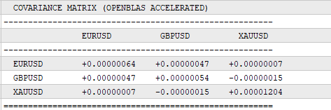
Read this image to understand the relationships between the assets. The diagonal entries —+0.00000064 for EURUSD, +0.00000054for GBPUSD, and +0.00001204 for XAUUSD — represent the individual variances (the asset's own volatility). By placing them within this grid structure, you can easily compare their individual behavior against their relationships with neighboring assets.

The off-diagonal entries reveal how the assets move in relation to one another:

• EURUSD and GBPUSD (+0.00000047): This value is large relative to both diagonal entries, immediately signaling a strong positive correlation between the two currency pairs.

• GBPUSD and XAUUSD (-0.00000015): Notice the negative sign. This tells you that GBPUSD and XAUUSD have a mild inverse relationship over this lookback window—when one tends to move up, the other tends to move slightly down.

• XAUUSD’s Independent Variance (+0.00001204): This value dwarfs all off-diagonal entries in its row, confirming that Gold's movements are largely driven by its own independent factors rather than by the same drivers moving the currency pairs.

Viewing the covariance matrix as a labeled grid makes these relationships immediately visible. Instead of working with an abstract mathematical object, we can inspect both the individual variances and the pairwise covariances directly from the journal output.

From Total Risk to Risk Components: The Case for Eigendecomposition

Here is the transition that defines Part 2's contribution to this series.

In Part 1, the covariance matrix was used to compute one number:

//--- Part 1 — the entire purpose of the matrix
  vector intermediate = cov_matrix.MatMul(w);
  double true_variance = w.Dot(intermediate);

This answered: how much total risk does the portfolio have? A single scalar. Useful, but it compresses all the information in the matrix into one figure.

The covariance matrix contains far more information than that scalar reveals. It encodes the complete structure of how the instruments relate to each other — and buried inside that structure are the underlying market factors driving the portfolio's risk. To extract those factors, we need eigenvalue decomposition.

Eigenvalue decomposition takes the covariance matrix and produces two outputs:

Eigenvalues tell us the variance capacity of each independent risk factor. Each eigenvalue is a number representing how much of the portfolio's total variance is accounted for by that factor. The sum of all eigenvalues equals the total portfolio variance — the same number Part 1 computed via wᵀ Σ w. The decomposition does not add new variance; it redistributes the existing variance across independent, orthogonal factors.

Eigenvectors tell us how each symbol loads onto each factor. An eigenvector is a set of coefficients — one per symbol — describing which direction in symbol-space this factor points. A large positive loading for EURUSD on Factor 1 means EURUSD moves strongly when Factor 1 moves. A near-zero loading means EURUSD barely participates in that factor.

The trading insight this produces is direct. Suppose Factor 1 has an eigenvalue that accounts for 75% of total portfolio variance. Suppose EURUSD loads at +0.61 on Factor 1 and GBPUSD loads at +0.65 on Factor 1. That tells you precisely: three quarters of your portfolio's risk comes from one underlying driver — broad US Dollar direction — and both of your currency pair positions are heavily exposed to it. They are not independent risks. They are two expressions of the same underlying bet.

The gap number told you the portfolio was riskier than expected. The eigenvalue decomposition tells you exactly why — and which instruments are the cause. That distinction is the transition from aggregate risk measurement to risk component analysis, and it is the foundation for everything this series builds in Parts 3 through 10.

The PrintEigenSpectrum Method: Calling .Eig()

The eigenvalue decomposition is performed inside PrintEigenSpectrum. The critical call is the native MQL5 .Eig() method:

 //--- Performs Eigendecomposition and generates organized risk factor spectrums
   void              PrintEigenSpectrum()
     {
      matrix eigenvectors;
      vector eigenvalues;

 //--- Executing native MQL5 OpenBLAS decomposition (Eigenvectors first, then Eigenvalues)
        if(!m_cov.Eig(eigenvectors, eigenvalues))
          {
           Print("ERROR: Eigenvalue decomposition failed.");
           return;
          }

The .Eig() method is called directly on m cov — the same matrix object built by Build() and verified by IsSymmetric(). It takes two output parameters: a matrix for the eigenvectors and a vector for the eigenvalues. The parameter order is critical: eigenvectors comes first, eigenvalues comes second. This order is defined by MQL5's native .Eig() method. Reversing them would compile without error but produce nonsensical output — eigenvalues stored in a matrix and eigenvectors stored in a vector would generate type mismatches or silent data corruption.

After a successful call, eigenvectors is a matrix where each column is one eigenvector. The column at index k contains the eigenvector corresponding to eigenvalues[k]. The eigenvalues vector contains one eigenvalue per factor. Together they completely describe the spectral decomposition of m_cov.

The .Eig() method is available for symmetric matrices — which a correctly computed covariance matrix always is, as our IsSymmetric() check confirms. It was introduced with the OpenBLAS integration in MetaTrader 5 build 4570 and is available in all current terminal versions. If your terminal predates build 4570, the method returns false and the error message will appear in the journal. Updating MetaTrader 5 to the current build resolves this immediately.

Sorting Eigenvalues: Largest Factor First

The .Eig() method does not guarantee any ordering of eigenvalues. To produce a consistently readable report with the dominant risk factor listed first, we sort using an index array:

 //--- Initialize index array for sorting risk shares from largest to smallest
      int idx[];
      ArrayResize(idx, n);
      for(int i = 0; i < n; i++) idx[i] = i;

      //--- Simple sorting loop (Bubble sort variant for sorting index mappings)
        for(int i = 0; i < n - 1; i++)
           for(int j = i + 1; j < n; j++)
              if(eigenvalues[idx[j]] > eigenvalues[idx[i]])
                {
                 int tmp = idx[i]; idx[i] = idx[j]; idx[j] = tmp;
                }

We sort an index array rather than the eigenvalues vector itself because eigenvectors and eigenvalues are linked: column k of eigenvectors corresponds to eigenvalues[k]. Sorting the eigenvalues vector directly would break that correspondence — the eigenvalue at position 0 would no longer match the eigenvector in column 0. By sorting the index array instead, we access both eigenvalues[idx[f]] and eigenvectors[s][idx[f]] using the same index f, preserving the link between each eigenvalue and its eigenvector throughout the report loop.

Printing the Risk Factor Report

With sorted indices in hand, the report loop prints each factor:

      double total_variance = 0.0;
      for(int i = 0; i < n; i++) total_variance += eigenvalues[i];

      PrintDivider("=");
      Print("  EIGENVALUE SPECTRUM — RISK FACTOR DECOMPOSITION");
      PrintDivider();
      PrintFormat("  Total Portfolio Variance: %.8f", total_variance);
      PrintDivider();

      //--- Print sorted factors alongside their respective asset loadings
        for(int f = 0; f < n; f++)
          {
           int    k   = idx[f];
           double ev  = eigenvalues[k];
           double pct = (total_variance > 0) ? (ev / total_variance) * 100.0 : 0.0;

           PrintFormat("  Factor %d | Eigenvalue: %+.8f | Risk Share: %.2f%%",
                       f + 1, ev, pct);

           for(int s = 0; s < m_size; s++)
              PrintFormat("    Loading on %-10s : %+.6f",
                          m_symbols[s], eigenvectors[s][k]);
           PrintDivider();
          }

total_variance is the sum of all eigenvalues. This is a mathematical property of eigendecomposition — the sum of all eigenvalues of a covariance matrix equals the matrix trace, which equals the sum of all individual variances. In practical terms, it means the percentage figures across all factors always sum to 100%, making the report self-consistent. If you sum the Risk Share percentages in the output and they do not add to 100%, something has gone wrong numerically.

For each factor f, the outer loop retrieves the sorted index k and computes the eigenvalue's percentage of total variance. The inner loop then prints each symbol's loading on this factor — accessed as eigenvectors[s][k], where s is the symbol row and k is the eigenvector column corresponding to this factor.

The loading values are the raw eigenvector components. Their sign and magnitude carry specific meaning. A loading near +1.0 or -1.0 means that symbol aligns strongly with this factor direction. A loading near 0.0 means the symbol is essentially orthogonal to this factor — it barely participates in this risk direction. When two symbols have large loadings of the same sign on the same factor, they are both heavily exposed to the same underlying market driver.

Finally, the concentration check:

 //--- Check dominant variance concentration metrics
      double factor1_pct = (total_variance > 0)
                           ? (eigenvalues[idx[0]] / total_variance) * 100.0 : 0.0;

      if(factor1_pct > 70.0)
         PrintFormat("  WARNING: Factor 1 holds %.2f%% of total variance. "
                     "Portfolio is CONCENTRATED.", factor1_pct);
      else
         PrintFormat("  RESULT: Risk distributed. Factor 1 = %.2f%% of variance.",
                     factor1_pct);

The 70% threshold is a practical rule of thumb. When one factor accounts for more than seventy percent of total variance, the portfolio is essentially one-dimensional — all positions are primarily expressing the same underlying market movement. The three separate volatility readings from Part 1 created the appearance of independence. The eigenvalue decomposition removes that appearance and replaces it with a fact.

Assembling OnStart()

With the class complete, OnStart() is concise and readable:

//+------------------------------------------------------------------+
//| Script entry point                                               |
//+------------------------------------------------------------------+
void OnStart()
  {
   PrintDivider("=");
   Print("  COVARIANCE MATRIX PRINTER — Part 2 Script");
   Print("  Measuring What Matters: Portfolio Risk Decomposition");
   PrintDivider("=");
   PrintFormat("  Symbols  : %s | %s | %s", Symbol1, Symbol2, Symbol3);
   PrintFormat("  Timeframe: %s", EnumToString(TF));
   PrintFormat("  Lookback : %d bars", LookbackBars);
   PrintDivider();

   vector returns[];
   ArrayResize(returns, 3);

   string symbols[3];
   symbols[0] = Symbol1;
   symbols[1] = Symbol2;
   symbols[2] = Symbol3;

//--- 1. Compute return data
   Print("Step 1: Computing log return series...");
   for(int i = 0; i < 3; i++)
     {
      if(!ComputeLogReturns(symbols[i], TF, LookbackBars, returns[i]))
         return;
     }
   PrintFormat("  Log returns computed: %d bars per symbol.", LookbackBars);
   PrintDivider();

//--- 2. Build and verify matrix
   Print("Step 2: Building covariance matrix...");
   CCovarianceMatrix cov_matrix(symbols, 3);
   if(!cov_matrix.Build(returns, 3))
     {
      Print("ERROR: Could not build covariance matrix. Exiting.");
      return;
     }
   Print("  Matrix built successfully.");


 //--- Validate structural symmetry properties from outline requirements
   if(cov_matrix.IsSymmetric())
      Print("  Computational Verification: Matrix symmetry test PASSED.");
   else
      Print("  WARNING: Structural asymmetry detected.");

   cov_matrix.PrintMatrix();

//--- 3. Execute decomposition
   Print("Step 3: Performing eigenvalue decomposition...");
   cov_matrix.PrintEigenSpectrum();

   PrintDivider("=");
   Print("  Script complete. See article Part 2 for full breakdown.");
   PrintDivider("=");
  }
//+------------------------------------------------------------------+

The completed OnStart() function focuses on orchestration rather than implementation. It collects return data, builds the covariance matrix, verifies its structure, prints the matrix, and performs the eigendecomposition. Each major operation is delegated to a dedicated class method, keeping the entry point compact and easy to follow. Part 2's OnStart() has a loop over an array. Adding a fourth symbol tomorrow means changing the array size from 3 to 4 and adding one input. Nothing else changes.

The sequence of three method calls — Build(), PrintMatrix(), PrintEigenSpectrum()— tells the complete story of Part 2 in three lines. Each method does one thing. Each adds one layer of understanding to the matrix that .Cov() produced.

Reading the Output: What the Numbers Mean

When you run CovarianceMatrixPrinter.mq5 on a live or demo account with default inputs, the eigenvalue spectrum section will show something structurally similar to this:

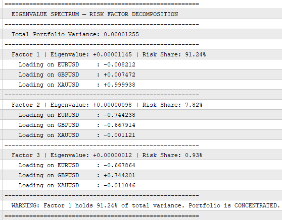
Read this as a story — and it is a striking one.

Factor 1 holds 91.24% of total portfolio variance. That is not a mild concentration warning — it means nine tenths of all the risk in this portfolio is coming from a single underlying factor. Look at the loadings: XAUUSD loads at +0.999938, which is essentially 1.0. EURUSD loads at -0.008212 and GBPUSD at +0.007472 — both near zero. Factor 1 is almost entirely Gold. XAUUSD's dominant variance of +0.00001204, which we saw in the matrix grid above, is so large relative to the two currency pairs that it consumes the overwhelming majority of the portfolio's risk budget. The two currency pairs are nearly invisible to Factor 1.

This is an immediate, actionable insight. If a trader holds equal positions in EURUSD, GBPUSD, and XAUUSD believing they are spreading risk across three instruments, the eigenvalue decomposition tells them plainly: 91% of their portfolio variance is Gold. The two currency pair positions are contributing almost nothing to the total risk picture compared to the Gold position.

Factor 2 holds 7.82% of variance. Here the loadings reverse — EURUSD loads at -0.744238 and GBPUSD at -0.667914, both significant and of the same sign, while XAUUSD loads at near zero (-0.001121). Factor 2 is the shared currency pair driver — broad US Dollar direction — which we might have expected to dominate if XAUUSD were not in the portfolio. With Gold present and its variance so much larger, the dollar factor is pushed into second place, accounting for less than 8% of total risk.

Factor 3 holds only 0.93% of variance. EURUSD loads at -0.667864 while GBPUSD loads at +0.744201 — opposite signs, similar magnitudes. This is the EUR/GBP differential: the minor directional divergence between the two currency pairs when they do not move perfectly together. At under 1% of total variance it is negligible in practice, but it is real and the decomposition captures it.

Part 2 tells you exactly why — not because of correlation between the currency pairs, but because one instrument (XAUUSD) is so much more volatile than the others that it dominates the entire portfolio's variance structure. That distinction matters enormously for position sizing: the correct response is not to reduce correlation but to reduce the Gold position size relative to the currency pairs until the factor risk shares reach a distribution the trader is comfortable with.

What This Means Going Forward

The practical implication for position sizing is direct. Factor 1 holds 91.24% of portfolio variance and is driven almost entirely by XAUUSD — which loads at +0.999938. Equal weighting across the three symbols means you have implicitly allocated over 91% of your effective risk budget to a single Gold-driven factor. The two currency pair positions, despite appearing as separate allocations, are contributing less than 9% of the portfolio's total variance combined. XAUUSD is not diversifying the portfolio — it is dominating it. The correct response is to significantly reduce the Gold position size relative to the currency pairs until the factor risk shares reach a balance the trader can consciously defend.

In Parts 5 and 6 of this series we will use the eigenvectors directly to compute position weights — allocating risk along independent factor directions rather than equally across symbol names. The CCovarianceMatrix class built in this article will be the component those parts import. The .Eig() output stored here will become the input to the weight calculation there.

For now, the single most important number to read from this output is the Factor 1 risk share. Above 70% means your portfolio is concentrated — your diversification is weaker than your position sizing assumes. Below 50% means your instruments are providing meaningful independent risk directions. That figure — the dominant eigenvalue's share of total variance — is the most informative risk metric this series produces, and it comes entirely from the matrix structure that Part 2 introduces.

Conclusion

Part 2 extends the foundation established in the previous article by transforming the covariance matrix from an intermediate calculation into an object that can be inspected, verified, and decomposed. Through the CCovarianceMatrix class, the matrix is stored, printed as a labeled grid, validated for symmetry, and analyzed using the native .Eig() method to reveal the independent factors driving portfolio risk.

The result is more than a covariance calculation. The matrix becomes an interpretable representation of portfolio structure, allowing traders to see how much each independent factor contributes to total variance and how each instrument loads onto those factors.

The ComputeLogReturns function carried forward unchanged from Part 1 is not just a convenience — it is the data layer on which this entire series is built. The CCovarianceMatrix class introduced in Part 2 is not just cleaner code — it is the reusable component that Parts 3 through 10 will import directly. The eigenvalue spectrum printed by PrintEigenSpectrum is not just a journal report — it is the first time the reader can see, named and quantified, the underlying factors driving their portfolio's risk.

In Part 3, we put the eigenvalues and eigenvectors produced here to a rigorous mathematical test. Using the spectral theorem — A = V Λ Vᵀ — we write a script called EigenRecomposer.mq5 that takes the eigenvectors and eigenvalues from Part 2's decomposition, constructs the diagonal matrix Λ using matrix.Diag(), executes the full triple matrix product V × Λ × Vᵀ via .MatMul() and .Transpose(), and subtracts the result from the original covariance matrix. The residual should be absolute zero — a reconstruction error at the level of 1×10⁻¹⁵ — proving that the three factors extracted in Part 2 captured the complete reality of the portfolio's risk structure with zero data loss.

Attached File: CovarianceMatrixPrinter.mq5

Next: Part 3 — The Reconstruction Engine: Validating Risk Footprints with Matrix Algebra