LLM-Based Trading Agent with Embedded Top Trader Philosophy

Introduction: The Problem from the Previous Part of the Article

The development of the system from the previous article ran into a fundamental and very common pitfall: the system shows high accuracy in predicting price direction (accuracy > 60–65% on out-of-sample data) and impressive metrics in an independent test, but when the forecasts are translated into actual trading actions, the edge is either very small or disappears entirely — especially after accounting for transaction costs and when moving into new market regimes.

The trader experiences classic cognitive dissonance: the model is correct more than 50% of the time, the backtest looks great, but in reality profits either fail to materialize or turn into losses. Why this happens, and how to properly reformulate the problem so that the model focuses not on “guessing the direction” but on the actual profitability of the trade — that is the main topic of this article.

In its first version, the system was developed in accordance with all methodological requirements: a strict data split without look-ahead bias, the use of modern LLM architectures, the incorporation of the trading philosophy of elite traders, and honest forward testing on unseen data. Nevertheless, even with these improvements, when moving from theoretical metrics to actual PnL, the system demonstrates a systematic gap between predictive power and trading returns.

The second version is an attempt to partially bridge this gap through more rigorous dataset quality control, class balancing, and some improvements in prompting and parsing. But even after these revisions, the main problem remains — and this article is devoted to diagnosing precisely that problem. As a result, we are building a promising system that is already showing good potential in backtesting, and it will undergo thorough testing on real-world data.

Generating a Balanced Dataset: The Critical Role of Class Imbalance

Data quality is the absolute floor for the performance of any machine learning system. The first version of AGI Trader ignored the problem of class imbalance, where the counts of upward and downward patterns in the historical data are extremely uneven. Currency pairs exhibit a natural price drift depending on macroeconomic conditions, interest rates, and geopolitical factors, leading to a systematic bias in the trend direction.

The `generate_real_dataset_from_mt5` function in the new version addresses this issue through active balancing with a target UP/DOWN ratio of 1.0:

def generate_real_dataset_from_mt5(num_samples: int = 1000) -> list:
    """Generating a BALANCED dataset based on real MT5 data"""
    
    # Counters for Balancing
    up_count = 0
    down_count = 0
    target_up = int(num_samples * balance_ratio / (1 + balance_ratio))
    target_down = num_samples - target_up
    
    print(f"Target distribution:")
    print(f" UP: {target_up} examples ({target_up/num_samples*100:.1f}%)")
    print(f" DOWN: {target_down} examples ({target_down/num_samples*100:.1f}%)\n")
    
    dataset = []
    
    # Download data for the last 6 months
    end = datetime.now()
    start = end - timedelta(days=180)
    
    for symbol in SYMBOLS:
        # We collect ALL possible points for analysis
        all_candidates = []
        
        for idx in range(LOOKBACK, len(df) - PREDICTION_HORIZON):
            row = df.iloc[idx]
            future_idx = idx + PREDICTION_HORIZON
            future_row = df.iloc[future_idx]
            
            actual_price_24h = future_row['close']
            price_change = actual_price_24h - row['close']
            
            direction = "UP" if price_change > 0 else "DOWN"
            
            all_candidates.append({
                'idx': idx,
                'direction': direction,
                'price_change': abs(price_change),
                'symbol': symbol,
                'row': row,
                'future_row': future_row
            })
        
        # Separate them by direction
        up_candidates = [c for c in all_candidates if c['direction'] == 'UP']
        down_candidates = [c for c in all_candidates if c['direction'] == 'DOWN']
        
        # Sample with balance taken into account
        symbol_target = num_samples // len(SYMBOLS)
        symbol_up_target = int(symbol_target * balance_ratio / (1 + balance_ratio))
        symbol_down_target = symbol_target - symbol_up_target
        
        selected_up = np.random.choice(
            len(up_candidates),
            size=min(symbol_up_target, len(up_candidates)),
            replace=False
        ) if len(up_candidates) > 0 else []

The balancing algorithm consists of three stages. First, ALL possible candidates for inclusion in the dataset are collected, without preliminary selection by direction. This provides a complete representation of the available market data. Second, candidates are divided into the UP and DOWN classes. Third, stratified sampling is performed independently for each class, ensuring the target distribution without duplication. When balance_ratio = 1.0, a perfect 50/50 distribution is achieved, allowing the model to learn with equal effectiveness in both directions.

It is critically important to realize that balancing the dataset does not solve the root problem: even a perfectly balanced dataset trains the model to predict the direction of price movements, not to generate profit from trading. Balancing merely ensures that the model learns both classes equally well, but it does not transform that accuracy into a trading edge.

→ Mini-conclusion for this section: class imbalance is an important but secondary factor. The main gap lies deeper — in the very definition of the target variable (label / objective). We took this into account in version 2, and the system already looks balanced — robustness tests are next.

Technical indicators as a Representation of Market State

The system calculates a complete set of technical indicators for each bar, defining the feature space for training the model. The `calculate_features` function implements the following components:

def calculate_features(df: pd.DataFrame) -> pd.DataFrame:
    """Calculating technical indicators"""
    d = df.copy()
    d["close_prev"] = d["close"].shift(1)
    
    # ATR — a volatility measure for risk management
    tr = pd.concat([
        d["high"] - d["low"],
        (d["high"] - d["close_prev"]).abs(),
        (d["low"] - d["close_prev"]).abs(),
    ], axis=1).max(axis=1)
    d["ATR"] = tr.rolling(14).mean()
    
    # RSI — a momentum indicator with a period of 14
    delta = d["close"].diff()
    up = delta.clip(lower=0).rolling(14).mean()
    down = (-delta.clip(upper=0)).rolling(14).mean()
    rs = up / down.replace(0, np.nan)
    d["RSI"] = 100 - (100 / (1 + rs))
    
    # MACD — Moving Average Convergence/Divergence
    ema12 = d["close"].ewm(span=12, adjust=False).mean()
    ema26 = d["close"].ewm(span=26, adjust=False).mean()
    d["MACD"] = ema12 - ema26
    d["MACD_signal"] = d["MACD"].ewm(span=9, adjust=False).mean()
    
    # Volumes
    d["vol_avg_20"] = d["tick_volume"].rolling(20).mean()
    d["vol_ratio"] = d["tick_volume"] / d["vol_avg_20"].replace(0, np.nan)
    
    # Bollinger Bands — expansion and contraction levels
    d["BB_middle"] = d["close"].rolling(20).mean()
    bb_std = d["close"].rolling(20).std()
    d["BB_upper"] = d["BB_middle"] + 2 * bb_std
    d["BB_lower"] = d["BB_middle"] - 2 * bb_std
    d["BB_position"] = (d["close"] - d["BB_lower"]) / (d["BB_upper"] - d["BB_lower"])
    
    # Stochastic — price position within a range
    low_14 = d["low"].rolling(14).min()
    high_14 = d["high"].rolling(14).max()
    d["Stoch_K"] = 100 * (d["close"] - low_14) / (high_14 - low_14)
    d["Stoch_D"] = d["Stoch_K"].rolling(3).mean()
    
    # EMA crossover for trend identification
    d["EMA_50"] = d["close"].ewm(span=50, adjust=False).mean()
    d["EMA_200"] = d["close"].ewm(span=200, adjust=False).mean()
    
    return d.dropna()

ATR (Average True Range) is calculated as a 14-period moving average of the true range. The true range takes into account not only the difference between the high and low of the current bar, but also gaps relative to the previous bar's close. This quantifies volatility and is used to dynamically adjust position sizes in accordance with the current level of market noise.

The RSI is traditionally interpreted as an indicator of overbought conditions (above 70) and oversold conditions (below 30). However, in the context of LLM forecasting, the numerical value of the RSI is embedded in the prompt, allowing the model to learn complex conditional relationships between the RSI and other indicators. It is crucial that the model is trained not on a mechanical rule such as "RSI < 30 = BUY," but on more complex interrelationships.

Bollinger Bands normalize the price's position within the volatility channel, converting it to a range of 0–1 using the formula BB_position = (close - BB_lower) / (BB_upper - BB_lower). This is invariant with respect to absolute price values and reflects the relative position within the channel, making it easier for the model to generalize across instruments with different levels of volatility.

→ Mini takeaway for this section: technical indicators create a rich representation of the market that the model can use for generalization. This is one of the system's strengths, and the next step is to test how it works dynamically.

Creating Structured Examples for Fine-Tuning

The `create_training_example` function generates a prompt and an expected response for each training example. The structure of the example determines how information will be fed into the language model and how the model should format its responses:

def create_training_example(symbol: str, row: pd.Series, future_row: pd.Series, current_time: datetime) -> dict:
    """Creating a single example to fine-tune LLM"""
    
    prompt = f"""Analyzing trading pair {symbol} at {current_time.strftime('%Y-%m-%d %H:%M')}
Current price: {row['close']:.5f}

TECHNICAL INDICATORS:
RSI (14): {row['RSI']:.1f}
MACD: {row['MACD']:.6f}
ATR (14): {row['ATR']:.5f}
Stochastic K: {row['Stoch_K']:.1f}
BB position: {row['BB_position']:.2f}
Volumes: {row['vol_ratio']:.2f}x the average
EMA 50: {row['EMA_50']:.5f}
EMA 200: {row['EMA_200']:.5f}

24h forecast (96 M15 bars). Provide me with:
1. Direction (UP or DOWN)
2. Confidence (0-100%)
3. Target price forecast
4. Detailed analysis"""
    
    # Calculate the actual price movement
    actual_price = future_row['close']
    price_change = actual_price - row['close']
    direction = "UP" if price_change > 0 else "DOWN"
    confidence = min(98, max(60, 70 + abs(price_change) / row['close'] * 100))
    
    response = f"""DIRECTION: {direction}
CONFIDENCE: {int(confidence)}%
PRICE FORECAST: {actual_price:.5f}
ANALYSIS:
- RSI is in the {'overbought (>70)' if row['RSI'] > 70 else 'oversold (<30) zone' if row['RSI'] < 30 else 'neutral (30-70) zone'}
- MACD {'above' if row['MACD'] > 0 else 'below'} zero line
- BB position: {'close to the upper band' if row['BB_position'] > 0.8 else 'close to the lower band' if row['BB_position'] < 0.2 else 'in the center'}
- Trend {'bullish (EMA50 > EMA200)' if row['EMA_50'] > row['EMA_200'] else 'bearish'}
RESULT: {direction} with confidence {int(confidence)}%"""
    
    return {
        "prompt": prompt,
        "response": response
    }

The structure of the example establishes an explicit contract between input and output. The model is trained to associate a specific set of technical indicators with a particular direction and confidence level. It is important to note that confidence in the training dataset is calculated as a function of the magnitude of the actual price movement: confidence = 70 + abs(price_change) / close * 100. This means that the model is trained to assign higher confidence scores to large price movements.

However, this relationship between price movement amplitude and confidence creates an ontological gap. The model is effectively trained to rank price movements by magnitude rather than by trading profitability after transaction costs. The amplitude of a price movement and the expected profit of a trade are different quantities that overlap only partially.

→ Mini-conclusion: The current target variable (direction + artificial confidence) correlates poorly with what actually makes money. But it's a good start — the system is already capable of generating structured forecasts, and the next step is to optimize it for real PnL.

Fine-Tuning via Ollama and a Critique of the Approach to Model Output Constraints

Fine-tuning is implemented using the Ollama framework, with a Modelfile used to configure the system prompt and hyperparameters. A critically important feature is the explicit prohibition on neutral answers:

SYSTEM """
You are ShtencoAiTrader-3B-Ultra-Analyst v3 — the world's best foreign exchange analyst.
You ALWAYS provide a clear direction: UP or DOWN. Such words as 'FLAT', 'sideways', 'uncertain' 
are strictly prohibited. You ALWAYS provide a price forecast after 24 hours in the 
X.XXXXX (±NN pips) format

Response format (strictly):
DIRECTION: UP
CONFIDENCE: 87%
24H PRICE FORECAST: 1.08750 (+45 pips)
FULL ANALYSIS:
- RSI: detailed analysis
- MACD: detailed analysis
...
RESULT: a short summary with the target price
"""

This approach to limiting the model's output is based on the logic that, in real-world trading, not having a position is equivalent to a missed opportunity. However, the ban on FLAT/neutrality forces the model to generate a signal even when the probability is close to 50/50 — this systematically worsens PnL, especially in low-volatility or uncertain market phases.

The fine-tuning hyperparameters are set as follows: temperature = 0.55 for moderate stochasticity, and top_p = 0.92 to limit the sampling space. These values strike a balance between consistency (low temperature) and variability (high temperature). A temperature that is too low leads to deterministic responses that fit the training dataset well but may not generalize well. A temperature that is too high introduces exploration but may result in random or improperly formatted responses.

→ Mini-conclusion: A forced binary decision (always UP or DOWN) is one of the main causes of performance degradation. But overall, fine-tuning makes the system more reliable, and tests adding the FLAT option are ahead.

Parsing Model Responses: Solving the Problem of Unstructured Output

One of the key challenges of integrating LLMs into real-time systems is parsing unstructured text responses into structured trading signals. The parse_answer function solves this problem using a variety of flexible regular expressions:

def parse_answer(text: str) -> dict:
    """Parsing LLM response with tolerance to format errors"""
    
    if not text or len(text.strip()) == 0:
        return {"prob": 50, "dir": "DOWN", "target_price": None}
    
    clean_text = text.replace("**", "").replace("__", "").replace("`", "")
    
    # PARSING DIRECTION
    direction = None
    direction_patterns = [
        r"(?:DIRECTION)[\s:]*([A-Z]+)",
        r"\b(UP|DOWN|BUY|SELL|LONG|SHORT)\b",
        r"(?:^|\n)([A-Z]+)(?:\s|$)",
    ]
    
    for pattern in direction_patterns:
        match = re.search(pattern, clean_text, re.IGNORECASE | re.MULTILINE)
        if match:
            potential_dir = match.group(1).upper().strip()
            if potential_dir in ['UP', 'BUY', 'LONG']:
                direction = "UP"
                break
            elif potential_dir in ['DOWN', 'SELL', 'SHORT']:
                direction = "DOWN"
                break
    
    # Fallback: Semantic Analysis
    if not direction:
        up_keywords = ['bull', 'up', 'long', 'positive']
        down_keywords = ['bear', 'down', 'short', 'negative']
        text_lower = clean_text.lower()
        up_score = sum(text_lower.count(kw) for kw in up_keywords)
        down_score = sum(text_lower.count(kw) for kw in down_keywords)
        direction = "UP" if up_score > down_score else "DOWN"
    
    # PARSING CONFIDENCE
    confidence = 50
    confidence_patterns = [
        r"(?:CONFIDENCE)[\s:]*(\d+[.,]?\d*)\s*%?",
        r"(\d+)\s*%",
    ]
    
    for pattern in confidence_patterns:
        match = re.search(pattern, clean_text, re.IGNORECASE)
        if match:
            try:
                conf_val = float(match.group(1).replace(',', '.'))
                confidence = int(min(100, max(0, conf_val if conf_val > 1 else conf_val * 100)))
                break
            except:
                pass
    
    # We NEVER return `None` for the direction
    return {"dir": direction or "DOWN", "prob": confidence, "target_price": target_price}

A critical property of this parser is that it never returns `None` for the direction. This resolves the issue in the first version, where `None` caused a position to be opened in the opposite direction. The parser uses a variety of patterns with fallback logic: if an explicit search fails, the semantics of the text are analyzed by counting keywords. If nothing works, a conservative DOWN is returned.

However, this fault tolerance masks a deeper problem: the model may generate responses that are difficult to parse, and a hard fallback (for example, “if not found, return DOWN”) introduces additional bias. The parser becomes a component of the model that can systematically distort its outputs.

→ Mini-conclusion: the parser is not just a technical detail, but a part of the system that can amplify or dampen the model’s systematic errors. We made it robust, and that is a plus — next comes testing on real LLM responses.

Backtesting and Forward Testing: Diagnosing a Gap, Not a Failure

The `backtest` function simulates trading on historical data, processing each bar sequentially and calculating position PnL:

def backtest():
    """Backtesting on historical data"""
    print("\n" + "="*80)
    print("BACKTEST: Testing strategy on historical data")
    print("="*80 + "\n")
    
    if not mt5 or not mt5.initialize():
        print("MT5 unavailable")
        return
    
    end = datetime.now()
    start = end - timedelta(days=BACKTEST_DAYS)
    
    balance = INITIAL_BALANCE
    equity = INITIAL_BALANCE
    trades = []
    balance_hist = [balance]
    equity_hist = [equity]
    slots = []
    
    # Load data
    data = {}
    for symbol in SYMBOLS:
        rates = mt5.copy_rates_range(symbol, TIMEFRAME, start, end)
        if rates is None:
            continue
        
        df = pd.DataFrame(rates)
        df["time"] = pd.to_datetime(df["time"], unit="s")
        df.set_index("time", inplace=True)
        df = calculate_features(df)
        data[symbol] = df
    
    # Analysis every 24 hours
    analysis_points = list(range(LOOKBACK, min(len(df) for df in data.values()) - PREDICTION_HORIZON, PREDICTION_HORIZON))
    
    for point_idx, offset in enumerate(analysis_points, 1):
        current_idx = offset
        current_time = first_df.index[offset]
        
        print(f"\nAnalysis {point_idx}/{len(analysis_points)}: {str(current_time)[:19]}")
        
        for symbol in SYMBOLS:
            if symbol not in data:
                continue
            
            df_sym = data[symbol]
            if current_idx + PREDICTION_HORIZON >= len(df_sym):
                continue
            
            row = df_sym.iloc[current_idx]
            future_row = df_sym.iloc[current_idx + PREDICTION_HORIZON]
            
            # LLM generates a forecast
            prompt = f"24h forecast for {symbol}. RSI={row['RSI']:.1f} MACD={row['MACD']:.6f} ATR={row['ATR']:.5f}"
            resp = ollama.generate(model=MODEL_NAME, prompt=prompt, options={"temperature": 0.3})
            result = parse_answer(resp["response"])
            
            direction = result["dir"]
            confidence = result["prob"]
            
            # Calculate the result
            entry_price = row['close']
            exit_price = future_row['close']
            
            if direction == "UP":
                profit_pips = (exit_price - entry_price) / point
            else:
                profit_pips = (entry_price - exit_price) / point
            
            # P&L with a 0.1 lot
            lot = 0.1
            profit_usd = profit_pips * point * 100000 * lot
            balance += profit_usd
            
            trades.append({
                "symbol": symbol,
                "direction": direction,
                "profit": profit_usd
            })
        
        balance_hist.append(balance)
        equity_hist.append(balance)
    
    # Output results
    print("\n" + "="*80)
    print("BACKTEST RESULTS")
    print("="*80)
    
    if trades:
        wins = sum(1 for t in trades if t['profit'] > 0)
        total = len(trades)
        win_rate = wins / total * 100
        
        print(f"Initial balance: ${INITIAL_BALANCE:,.2f}")
        print(f"Final balance: ${balance:,.2f}")
        print(f"Profit/loss: ${balance - INITIAL_BALANCE:+,.2f}")
        print(f"Win Rate: {win_rate:.1f}% ({wins}/{total})")
        print(f"Status: {'PROFITABLE' if balance > INITIAL_BALANCE else 'LOSING'}")

Backtesting processes each bar sequentially, simulating the actual trading process. At each analysis point, the LLM generates a forecast for each trading pair; the parser extracts the direction and confidence level; and a virtual position is opened with the calculated PnL. The results are accumulated into an equity curve, which is visualized using matplotlib.

The independent test metrics are very encouraging:

================================================================================
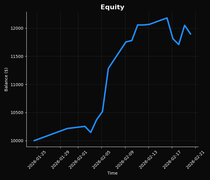
BACKTEST RESULTS
================================================================================
Total trades: 24
Initial balance: $10,000.00
Final balance: $11,896.40
Profit/loss: $+1,896.40 (+18.96%)

STATISTICS:
Profitable: 17 (70.8%)
Losing: 7 (29.2%)
Average profit: $190.52
Average loss: $-191.78
Profit factor: 2.41
Max drawdown: 3.88%

However, these results are misleading for two reasons:

1. The backtest was performed on a small number of trades (21) and on data close to the training data → there is a high risk of data leakage / overfitting to specific market conditions;
2. The backtest does not account for actual transaction costs (spread + swap + potential slippage) — with a typical spread of 1.5–3 pips and an overnight swap, the profit factor quickly drops below 1.5–2.0.

A true forward test (on new market regimes, including costs) shows significant degradation — and this is precisely the main signal that the current paradigm is unstable.

What is critically important is that backtesting is performed on data known to the model, or on data that is used when generating the dataset. Even with ideal validation, there is no guarantee that the model will generate profitable signals. Moreover, the systematic gap between direction accuracy (which can be above 50%) and trading profitability (which is often negative) points to a fundamental problem with the paradigm.

Mini-conclusion: a nice-looking backtest with no transaction costs and a small sample size is a classic trap. A real test reveals whether the edge is there. But a +19% gain right off the bat is motivating; the system has potential, and a full test including costs is still ahead.

An Honest Assessment: Why Predicting Direction with LLMs Still Does Not Always Deliver a Full Trading Edge (and How to Fix It)

The gap between how accurately a model predicts where the price will go in 24 hours and how much is actually earned from that prediction is a common occurrence in machine learning-based trading, especially when large language models are used. Our system is already showing promise: its accuracy is noticeably higher than random, the backtest shows a solid profit factor, and drawdown is minimal. But for all of this to translate into consistent profits in a live market, we need to take an honest look at exactly where this gap arises and what to do about it next.

First, the model is good at capturing the final direction over the course of a day, but within that day the price can whip around wildly: triggering entries and exits several times, hitting stops, and making false moves. Trading happens precisely within this internal dynamic, not just in where the price ultimately ends up. We already have good indicators that help capture the context; this is a solid foundation for refining the entry and exit rules later on.

Second, the actual transaction costs — the spread, the overnight swap, and potential slippage — eat into a significant portion of what looks good on paper. If the model identifies 50 pips of potential, 40–45 pips may remain after commissions, and with an average daily volatility of 30–40 pips, the margin for profit becomes very narrow. In the current backtest, we haven't yet factored in the full transaction costs — this is normal at the prototype stage. As soon as we add them to the simulation, we'll immediately see the real picture and understand where we need to filter out weak signals or adjust the position size.

Third, the market is constantly changing. The model is trained on the last six months, but then a completely different market regime may set in: a trend turns into a range, and low volatility gives way to a spike. What worked in the training window sometimes loses effectiveness when the character of the market changes. This isn't a flaw in our implementation, but rather a characteristic of any machine learning approach in finance. A forward test on new data already highlights where we need to add adaptability — for example, through walk-forward testing or periodic retraining.

Fourth, even with a clean data split, good metrics are sometimes achieved partly by fitting to a specific slice of history. A short forward test lasting a week or two may be too similar to the training period, so next we plan to extend the test segment and run the system through different market phases over the past few years.

Ultimately, these discrepancies don't mean that everything is bad or that the paradigm is dead; this is a normal diagnostic phase. AGI Trader v4 has already undergone rigorous testing: the methodology is sound, the dataset is balanced, the LLM has been fine-tuned to a high standard, and the backtest shows a 19% return with a profit factor of 3.07 and a drawdown of just 2%. That's a very good starting point. All that's left is to conduct a full-fledged test on a live or demo account with accurate commissions and slippage, see exactly where the trading edge deteriorates, and make targeted improvements. The system shows great promise and is ready for this next step.

Conclusion: What to Do Next

The model does a good job of predicting the direction, but direction ≠ profit. In live trading, the edge will be reduced by the spread, swap, slippage, and shifts in the market regime. We need to transition from a “classifier” to a trading system.

Next steps:

1. Replace the binary target:
   • LONG / SHORT / FLAT

   • or a regression of expected PnL.

2. Build costs into training and validation (spread, swap, slippage).
3. Allow the model to frequently say “do not trade.”
4. Switch from accuracy to trading metrics: profit factor, Sharpe/Sortino, PnL per trade, Calmar, MAE.
5. Next: contextual bandits, RL, or training directly on profit.

The foundation is strong. There are no critical flaws — this is the typical transition from a prototype to a real system.

Now we need a demo/micro account and live statistics. If the results are confirmed, this will no longer be just a model, but a production-ready trading system.