
Data Science and ML (Part 48): Are Transformers a Big Deal for Trading?

Contents
- What is a Transformer model?
- Background
- Transformer model architecture
- Temporal Fusion Transformer (TFT) model
- Preparing Data for the TFT model
- Training the Temporal Fusion Transformer
- Finding the best parameters for Temporal Fusion Transformer model
- Making a trading robot out of the TFT model
- Conclusion
What is a Transformer Model?
In deep learning, a transformer is an artificial neural network architecture based on the multi-head attention mechanism. This architecture was first introduced in the 2017 paper “Attention Is All You Need,” authored by eight researchers at Google. The paper presented a new model built upon the attention mechanism originally proposed by Bahdanau et al. in 2014, and it is widely regarded as a foundational contribution to modern artificial intelligence.
Transformers have achieved remarkable achievements across diverse domains. In the context of Natural Language Processing (NLP), they have proven their abilities in language translation, sentiment analysis, and text summarization. Expanding their applicability to image processing, they have been adeptly tailored for vision tasks, demonstrating success in image classification and object detection. Furthermore, their effectiveness extends to time series analysis, where their unique ability to capture long-range dependencies renders them suitable for predicting sequential data, demonstrated in tasks such as forecasting stock prices or predicting weather patterns.
The term transformer used in this article refers to a family of architectures based on attention, not a single fixed model.
Transformers are a family of neural network architectures built around attention mechanisms rather than recurrence. Unlike traditional sequential models, they allow each element in a sequence to directly attend to all others, enabling efficient modeling of long-range dependencies and parallel computation during training.
While originally developed for natural language processing, Transformer variants have since been adapted to vision and time-series tasks, often with architectural modifications to account for domain-specific constraints such as known future inputs, multi-horizon prediction, and limited data availability.
Background
In the field of Natural Language Processing (NLP), sequential models such as RNNs and LSTMs have been widely adopted. These models have demonstrated strong performance in tasks like machine translation and language modeling. However, they possess inherent structural limitations when processing sequential inputs.
Primary limitations are as follows:

A structure of the existing sequential model
Long Computation Time
Conventional sequential models typically utilize information from previous time steps as input to interpret the current time step. Like the example shown in Figure 1, the sequential dependency creates a structure where hidden features are processed one step at a time. Consequently, computation time scales linearly with input length, which becomes increasingly inefficient as sequences grow longer.
Difficulty in Capturing Long-Range Dependencies
Due to their sequential nature, Recurrent Neural Network (RNN) models struggle to capture dependencies between distant elements in a sequence. Although architectures like LSTM and GRU have been introduced to alleviate this issue, they still rely on fixed-size hidden state representations, which limit their ability to effectively process extremely long sequences.
Developers at Google proposed a Transformer model that eliminates recurrence entirely and instead relies on an attention mechanism to establish global dependencies between input and output elements. This architecture was aimed to effectively addresses the aforementioned limitations and enhance the model’s scalability and efficiency, though modern variants may reintroduce it for specific domains such as time series.
Transformer Model Architecture
![]()
Self-Attention Mechanism
Unlike traditional Recurrent Neural Networks (RNNs) and Long Short-Term Memory (LSTMs) neural networks, transformers rely on a self-attention mechanism that enables the model to weigh the importance of different parts of the input sequence when making predictions.
Parallelization
Transformers allow parallelization during training, though some variants remain sequential during inference, making it more efficient than sequential models like RNNs. This results in faster training times.
Encoder-Decoder Structure
The model is composed of an encoder and a decoder. The encoder processes the input sequence, capturing contextual information, while the decoder generates the output sequence.
Multi-Head Attention
The self-attention mechanism is extended with multiple heads, allowing the model to focus on different aspects of the input sequence simultaneously. This enhances its ability to capture complex relationships.
Unlike fixed-size hidden states, attention allows the model to dynamically select relevant information from any point in the sequence.
Positional Encoding
Transformers do not inherently understand the order of the input sequence. To address this, positional encodings are added to the input embeddings, providing information about the positions of tokens in the sequence.
Again, the term Transformers used several times in this article doesn't refer to a single model; the architecture can differ significantly for different types of transformer models. For example:
| Model | Architecture | Primary Use / Domain |
|---|---|---|
| Original Transformer | Encoder-Decoder. | Machine translation, sequence-to-sequence tasks. |
| BERT (Bidirectional Encoder Representations from Transformers) | Encoder only. | Text understanding (classification, NER, embeddings) |
| GPT (Generative Pre-trained Transformer) | Decoder only. | Text generation, language modeling, code generation. |
| ViT (The Vision Transformer) | Encoder only. | Image classification, vision representation learning. |
| TFT (Temporal Fusion Transformer) | Hybrid (LSTM + Attention) | Time-series forecasting, financial and business data. |
More information about how transformers are composed and more can be found in the reference section, at the end of this article.
Out of all transformer models, the Temporal Fusion Transformer (TFT) is the one suitable for time series forecasting. In this article, we are going to discuss what it is, create one, and how we can use one to make forecasts on the market.
Temporal Fusion Transformer (TFT) Model
By definition;
A Temporal Fusion Transformer (TFT) is a state-of-the-art, attention-based deep learning model designed for multi-horizon time-series forecasting.
Introduced by Google and researchers at the University of Oxford back in 2021, it is designed to provide high-performance, interpretable predictions by combining LSTM-based (long short-term memory), encoder-decoder components with self-attention mechanisms.
For more information about its theory and architecture, see this article: https://medium.com/dataness-ai/understanding-temporal-fusion-transformer-9a7a4fcde74b
Let us implement this model using the PyTorch-forecasting framework.
We start by installing all the dependencies used in this project (requirements.txt file is found inside the attached zip file at the end of this article) in your Python virtual environment.
pip install -r requirements.txt
Preparing Data for the TFT Model
We start by importing data from the MetaTrader 5 terminal.
import MetaTrader5 as mt5

# Get rates from the MetaTrader5 app

if not mt5.initialize():
    print("initialize() failed, error code =", mt5.last_error())
    quit()

symbol = "EURUSD"
rates = mt5.copy_rates_from_pos(symbol, mt5.TIMEFRAME_M15, 0, 10000)
rates_df = pd.DataFrame(rates)

rates_df["time"] = pd.to_datetime(rates_df["time"], unit="s")
data = pd.concat([rates_df, get_features(rates_df)], axis=1)
Feature Engineering
We can't use all the features received; let's drop the ones we think are unnecessary.
rates_df.drop(columns=[
            "spread",
            "real_volume"
        ], inplace=True)
The remaining features after this operation aren't sufficient either, let's introduce new features to our DataFrame.
Below is a simple class to help us introduce various features (feature engineer new variables):
features.py
- Date and time-based features
features.py
import pandas as pd
from ta.trend import sma_indicator, ema_indicator, macd_diff, macd_signal
from ta.momentum import stochrsi_k, stochrsi_d, rsi
from ta.volatility import bollinger_hband, bollinger_lband

class FeatureEngineer:

    # date/time features

    @staticmethod
    def hour(date_series: pd.Series) -> pd.Series:
        return date_series.dt.hour

    @staticmethod
    def dayofweek(date_series: pd.Series) -> pd.Series:
        return date_series.dt.dayofweek

    @staticmethod
    def dayofmonth(date_series: pd.Series) -> pd.Series:
        return date_series.dt.day

    @staticmethod
    def month(date_series: pd.Series) -> pd.Series:
        return date_series.dt.month
- Trend following indicators
    # trend following indicators

    @staticmethod
    def sma(price: pd.Series, window: int=20) -> pd.Series:
        return sma_indicator(price, window)

    @staticmethod
    def ema(price: pd.Series, window: int=20) -> pd.Series:
        return ema_indicator(price, window)

    @staticmethod
    def macd_diff(price: pd.Series, window_slow: int=26, window_fast: int=12, window_signal: int=9) -> pd.Series:
        return macd_diff(price, window_slow=window_slow, window_fast=window_fast, window_sign=window_signal)

    @staticmethod
    def macd_signal(price: pd.Series, window_slow: int=26, window_fast: int=12, window_signal: int=9) -> pd.Series:
        return macd_signal(price, window_slow=window_slow, window_fast=window_fast, window_sign=window_signal
- Momentum indicators
    # momentum indicators

    @staticmethod
    def rsi(price: pd.Series, window: int=14) -> pd.Series:
        return rsi(price, window)

    @staticmethod
    def stochrsi_k(price: pd.Series, window: int=14, smooth1: int=3, smooth2: int=3) -> pd.Series:
        return stochrsi_k(price, window=window, smooth1=smooth1, smooth2=smooth2)

    @staticmethod
    def stochrsi_d(price: pd.Series, window: int=14, smooth1: int=3, smooth2: int=3) -> pd.Series:
        return stochrsi_d(price, window=window, smooth1=smooth1, smooth2=
- Volatility indicators
    # volatility indicators

    @staticmethod
    def bollinger_hband(price: pd.Series, window: int=20, window_dev: int=2) -> pd.Series:
        return bollinger_hband(price, window=window, window_dev=window_dev)

    @staticmethod
    def bollinger_lband(price: pd.Series, window: int=20, window_dev: int=2) -> pd.Series:
        return bollinger_lband(price, window=window, window_dev=window_dev)
We call methods in this class in a single static function called get_all from the same class.
    @staticmethod
    def get_all(data: pd.DataFrame) -> pd.DataFrame:

        return pd.DataFrame({
            "hour": FeatureEngineer.hour(data["time"]),
            "dayofweek": FeatureEngineer.dayofweek(data["time"]),
            "dayofmonth": FeatureEngineer.dayofmonth(data["time"]),
            "month": FeatureEngineer.month(data["time"]),
            "sma_20": FeatureEngineer.sma(data["close"]),
            "ema_20": FeatureEngineer.ema(data["close"]),
            "macd_diff": FeatureEngineer.macd_diff(data["close"]),
            "macd_signal": FeatureEngineer.macd_signal(data["close"]),
            "rsi": FeatureEngineer.rsi(data["close"]),
            "stochrsi_k": FeatureEngineer.stochrsi_k(data["close"]),
            "stochrsi_d": FeatureEngineer.stochrsi_d(data["close"]),
            "bollinger_hband": FeatureEngineer.bollinger_hband(data["close"]),
            "bollinger_lband": FeatureEngineer.bollinger_lband(data["close"]),
        })
We use this class to obtain a new Pandas-DataFrame full of features.
new_features = features.FeatureEngineer.get_all(rates_df)
Outputs.
(.env) C:\Users\Omega Joctan\OneDrive\mql5 articles\Data Science and ML\Part 48\TFT>python train.py
      hour  dayofweek  dayofmonth  month    sma_20    ema_20  macd_diff  macd_signal        rsi  stochrsi_k  stochrsi_d  bollinger_hband  bollinger_lband
0       20          3          21      8       NaN       NaN        NaN          NaN        NaN         NaN         NaN              NaN              NaN
1       20          3          21      8       NaN       NaN        NaN          NaN        NaN         NaN         NaN              NaN              NaN
2       20          3          21      8       NaN       NaN        NaN          NaN        NaN         NaN         NaN              NaN              NaN
3       20          3          21      8       NaN       NaN        NaN          NaN        NaN         NaN         NaN              NaN              NaN
4       21          3          21      8       NaN       NaN        NaN          NaN        NaN         NaN         NaN              NaN              NaN
...    ...        ...         ...    ...       ...       ...        ...          ...        ...         ...         ...              ...              ...
9985    20          4          16      1  1.160491  1.160265  -0.000107    -0.000404  41.591063    0.303937    0.316652         1.162598         1.158383
9986    20          4          16      1  1.160384  1.160213  -0.000068    -0.000421  43.685146    0.499779    0.367431         1.162418         1.158349
9987    20          4          16      1  1.160269  1.160151  -0.000047    -0.000433  42.436779    0.698607    0.500775         1.162214         1.158323
9988    21          4          16      1  1.160154  1.160067  -0.000046    -0.000444  40.194753    0.774743    0.657710         1.162051         1.158257
9989    21          4          16      1  1.160052  1.160010  -0.000026    -0.000450  42.452830    0.687333    0.720228         1.161864         1.158240

[9990 rows x 13 columns]
We then combine both DataFrames to form a larger one that we are going to use for the final model training.
data = pd.concat([rates_df, new_features], axis=1) # concatenate dataframes
Outputs.
                    time     open     high      low    close  tick_volume  ...  macd_signal        rsi  stochrsi_k  stochrsi_d  bollinger_hband  bollinger_lband
0    2025-08-21 20:00:00  1.16112  1.16171  1.16112  1.16170          642  ...          NaN        NaN         NaN         NaN              NaN              NaN
1    2025-08-21 20:15:00  1.16170  1.16173  1.16126  1.16136          557  ...          NaN        NaN         NaN         NaN              NaN              NaN
2    2025-08-21 20:30:00  1.16136  1.16167  1.16129  1.16158          414  ...          NaN        NaN         NaN         NaN              NaN              NaN
3    2025-08-21 20:45:00  1.16158  1.16187  1.16149  1.16151          513  ...          NaN        NaN         NaN         NaN              NaN              NaN
4    2025-08-21 21:00:00  1.16151  1.16152  1.16103  1.16106          473  ...          NaN        NaN         NaN         NaN              NaN              NaN
...                  ...      ...      ...      ...      ...          ...  ...          ...        ...         ...         ...              ...              ...
9985 2026-01-16 20:15:00  1.15911  1.15954  1.15905  1.15951          407  ...    -0.000404  41.591063    0.303937    0.316652         1.162598         1.158383
9986 2026-01-16 20:30:00  1.15951  1.15973  1.15936  1.15972          289  ...    -0.000421  43.685146    0.499779    0.367431         1.162418         1.158349
9987 2026-01-16 20:45:00  1.15972  1.15994  1.15955  1.15956          447  ...    -0.000433  42.436779    0.698607    0.500775         1.162214         1.158323
9988 2026-01-16 21:00:00  1.15956  1.15967  1.15921  1.15927          457  ...    -0.000444  40.194753    0.774743    0.657710         1.162051         1.158257
9989 2026-01-16 21:15:00  1.15927  1.15958  1.15915  1.15947          290  ...    -0.000450  42.452830    0.687333    0.720228         1.161864         1.158240

[9990 rows x 19 columns]
Making the Target variable
A typical supervised machine learning requires a target variable; a variable that a model has to predict using other features (predictors).
Since this is a time series problem, let's use returns as a target variable.
data["returns"] = data["close"].pct_change()
Creating a Time series Dataset Object
PyTorch-forecasting requires data for a model to be stored in an object called TimeSeriesDataset.
We need a column called time_idx in the DataFrame before assigning it to the TimeSeriesDataset object.
data["time_idx"] = data.index
data.drop(columns=["time"], inplace=True)
time_idx (str) – integer-typed column denoting the time index within data. This column is used to determine the sequence of samples. If there are no missing observations, the time index should increase by +1 for each subsequent sample. The first time_idx for each series does not necessarily have to be 0, but any value is allowed.
Once the column time_idx is introduced to a DataFrame, the original column containing time (datetime) has to be dropped (TFT doesn't use datetime variables directly).
data.drop(columns=["time"], inplace=True)
max_prediction_length = 6
max_encoder_length = 24
training_cutoff = data["time_idx"].max() - max_prediction_length

training = TimeSeriesDataSet(
    data[lambda x: x.time_idx <= training_cutoff],
    time_idx="time_idx",
    target="returns",
    group_ids=["symbol"],
    min_encoder_length=max_encoder_length // 2,  # keep encoder length long (as it is in the validation set)
    max_encoder_length=max_encoder_length,
    min_prediction_length=1,
    max_prediction_length=max_prediction_length,
    static_categoricals=["symbol"],
    # time_varying_known_categoricals=[],

    time_varying_known_reals=[
                            "hour",
                            "dayofweek",
                            "dayofmonth",
                            "month",
                            "time_idx",
                            "stochrsi_k",
                            "stochrsi_d",
                            "rsi",
                            "macd_diff",
                            ],

    time_varying_unknown_categoricals=[],
    time_varying_unknown_reals=[
        "open",
        "high",
        "low",
        "close",
        "tick_volume",
        "ema_20",
        "sma_20",
        "bollinger_hband",
        "bollinger_lband"
    ],

    target_normalizer=GroupNormalizer(
        groups=["symbol"], transformation="softplus"
    ),  # use softplus and normalize by group

    add_target_scales=True,
    add_encoder_length=True,
)
This object takes many variables, below table describes a few of those, Read more.
| Variable | Description |
|---|---|
| max_encoder_length | How much past the model is allowed to look at. |
| max_prediction_length | How far into the future the model must predict. |
| time_varying_known_reals | This is a list of continuous variables that change over time and are known in the future. We have selected stationary indicators we have in our DataFrame alongside time features. |
| time_varying_unknown_reals | This should be a list of continuous variables that are not known in the future and change over time. Target variables should be included here if real. For this, we've selected features such as open, high, low, close, etc. Features we are uncertain about their values in the future. |
| group_ids | A list of column names identifying a time series instance within data; This means that the group_ids identify a sample together with the time_idx. If you have only one timeseries, set this to the name of the column that is constant. Since we only have one symbol collected in our Pandas DataFrame, the only group we assign is the current symbol. data["symbol"] = "EURUSD"Groups might represent time series data from different instruments (symbols) and timeframes. |
We create the validation data by mimicking the training object.
#  (predict=True) which means to predict the last max_prediction_length points in time for each series

validation = TimeSeriesDataSet.from_dataset(
    training, data, predict=True, stop_randomization=True
)
Finally, we create PyTorch data loaders for both the training and validation data (dataloaders are suitable for feeding data into the models).
batch_size = 128  # set this between 32 to 128
train_dataloader = training.to_dataloader(
    train=True, batch_size=batch_size, num_workers=0
)
val_dataloader = validation.to_dataloader(
    train=False, batch_size=batch_size * 10, num_workers=0
)
Training the Temporal Fusion Transformer
We train our model with PyTorch Lightning, below is a Lightning trainer for the training task.
pl.seed_everything(42) # random seed for reproducibility

lr_logger = LearningRateMonitor()  # log the learning rate
logger = TensorBoardLogger("lightning_logs")  # logging results to a tensorboard

# configure network and trainer
early_stop_callback = EarlyStopping(
    monitor="val_loss", min_delta=1e-4, patience=10, verbose=False, mode="min"
)

trainer = pl.Trainer(
    max_epochs=50,
    accelerator="cpu",
    enable_model_summary=True,
    gradient_clip_val=0.1,
    limit_train_batches=50,  # comment in for training, running validation every 30 batches
    # fast_dev_run=True,  # comment in to check that networkor dataset has no serious bugs
    callbacks=[lr_logger, early_stop_callback],
    logger=logger,
)
Since we have no way of knowing the correct learning rate for our model, let's find one.
We create an instance of the TFT model to be used for finding the best learning rate.
tft = TemporalFusionTransformer.from_dataset(
    training,
    # not meaningful for finding the learning rate but otherwise very important
    learning_rate=0.03,
    hidden_size=8,  # most important hyperparameter apart from learning rate
    # number of attention heads. Set to up to 4 for large datasets
    attention_head_size=2,
    dropout=0.1,  # between 0.1 and 0.3 are good values
    hidden_continuous_size=8,  # set to <= hidden_size
    loss=metrics.QuantileLoss(),
    optimizer="ranger",
    # reduce learning rate if no improvement in validation loss after x epochs
    # reduce_on_plateau_patience=1000,
)
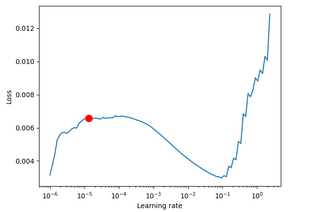
Finding an optimal learning rate.
res = Tuner(trainer).lr_find(
    tft,
    train_dataloaders=train_dataloader,
    val_dataloaders=val_dataloader,
    max_lr=10.0,
    min_lr=1e-6,
)

optimal_lr = res.suggestion()

print(f"suggested learning rate: {optimal_lr}")
fig = res.plot(show=False, suggest=True)

plots_path = os.path.join(outputs_dir, "Plots")
os.makedirs(plots_path, exist_ok=True)

fig.savefig(os.path.join(plots_path, "lr_finder.png"))
Outputs.
Finding best initial lr:  91%|█████████████████████████████████████████████████████████████████████████████████████████████▋         | 91/100 [00:41<00:04,  2.20it/s]
LR finder stopped early after 91 steps due to diverging loss.
Restoring states from the checkpoint path at C:\Users\Omega Joctan\OneDrive\mql5 articles\Data Science and ML\Part 48\TFT\.lr_find_6df0be87-4347-4325-98f1-3a2b5a244c46.ckpt
Restored all states from the checkpoint at C:\Users\Omega Joctan\OneDrive\mql5 articles\Data Science and ML\Part 48\TFT\.lr_find_6df0be87-4347-4325-98f1-3a2b5a244c46.ckpt
Learning rate set to 1.3182567385564071e-05
suggested learning rate: 1.3182567385564071e-05
With an optimal learning rate obtained, we create a new model instance and train it with such a learning rate value.
tft = TemporalFusionTransformer.from_dataset(
    training,
    learning_rate=optimal_lr,
    hidden_size=16,
    attention_head_size=2,
    dropout=0.1,
    hidden_continuous_size=8,
    loss=metrics.QuantileLoss(),
    log_interval=10,  # uncomment for learning rate finder and otherwise, e.g., to 10 for logging every 10 batches
    optimizer="ranger",
    reduce_on_plateau_patience=4,
)

print(f"Number of parameters in network: {tft.size() / 1e3:.1f}k")

trainer.fit(
    tft,
    train_dataloaders=train_dataloader,
    val_dataloaders=val_dataloader,
)

tft_predictions = tft.predict(val_dataloader, return_y=True)
print("TFT MAE: ", metrics.MAE()(tft_predictions.output, tft_predictions.y))
Outputs.
Epoch 4: 100%|██████████████████████████████████████████| 50/50 [01:04<00:00,  0.77it/s, v_num=1, train_loss_step=0.000846, val_loss=0.0013, train_loss_epoch=0.00092]`Trainer.fit` stopped: `max_epochs=5` reached.
Epoch 4: 100%|██████████████████████████████████████████| 50/50 [01:05<00:00,  0.77it/s, v_num=1, train_loss_step=0.000846, val_loss=0.0013, train_loss_epoch=0.00092]
💡 Tip: For seamless cloud uploads and versioning, try installing [litmodels](https://pypi.org/project/litmodels/) to enable LitModelCheckpoint, which syncs automatically with the Lightning model registry.
GPU available: False, used: False
TPU available: False, using: 0 TPU cores
TFT MAPE:  tensor(1.2644)+
Let's visualize predictions made by the model against the real values to get a glimpse of where the model's predictions stand compared to the true (original) values.
best_model_path = trainer.checkpoint_callback.best_model_path
best_tft = TemporalFusionTransformer.load_from_checkpoint(best_model_path)

# raw predictions are a dictionary from which all kinds of information, including quantiles, can be extracted
raw_predictions = best_tft.predict(
    val_dataloader, mode="raw", return_x=True, trainer_kwargs=dict(accelerator="cpu")
)

n = raw_predictions.output.prediction.shape[0]
print(f"Plotting {n} predictions...")

for idx in range(n):
    fig = best_tft.plot_prediction(
        raw_predictions.x,
        raw_predictions.output,
        idx=idx,
        add_loss_to_title=True
    )

    fig.savefig(os.path.join(plots_path, f"tft_prediction_{idx}.png"))
    plt.close(fig=fig)
Outputs.
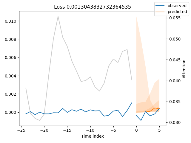
The predicted values seem close to the original values.
The MAE metric means nothing without a comparison; we have to know where our model stands among others. Let's find out using a baseline model.
A Baseline Model
This is a model that uses the last known target value to make a prediction. It gives us a simple benchmark that we want to outperform.
baseline_predictions = Baseline().predict(val_dataloader, return_y=True)
print("Baseline model MAE: ",metrics.MAE()(baseline_predictions.output, baseline_predictions.y))
After running the script once more, the TFT model was twice as accurate as a Baseline model.
TFT MAE:  tensor(0.0002)
Baseline model MAE:  tensor(0.0004)
Finding the Best Parameters for Temporal Fusion Transformer Model
Since a transformer model is a neural network-based model (has a Long Short-Term Memory (LSTM) at its core), just like any other neural network models, they are sensitive to hyperparameters.
To get the best out of them, we need the right set of hyperparameters for a particular problem the model is trying to solve.
According to the documentation:
Hyperparamter tuning with optuna is directly built into PyTorch-forecasting. We can use the optimize_hyperparameters() function to optimize the TFT’s hyperparameters.
For example:
import pickle

from pytorch_forecasting.models.temporal_fusion_transformer.tuning import optimize_hyperparameters

# create study
study = optimize_hyperparameters(
    train_dataloader,
    val_dataloader,
    model_path="optuna_test",
    n_trials=200,
    max_epochs=50,
    gradient_clip_val_range=(0.01, 1.0),
    hidden_size_range=(8, 128),
    hidden_continuous_size_range=(8, 128),
    attention_head_size_range=(1, 4),
    learning_rate_range=(0.001, 0.1),
    dropout_range=(0.1, 0.3),
    trainer_kwargs=dict(limit_train_batches=30),
    reduce_on_plateau_patience=4,
    use_learning_rate_finder=False,  # use Optuna to find ideal learning rate or use in-built learning rate finder
)

# save study results - also we can resume tuning at a later point in time
with open("test_study.pkl", "wb") as fout:
    pickle.dump(study, fout)

# show best hyperparameters
print(study.best_trial.params)
Unlike other Python frameworks for machine learning, such as scikit-learn and Keras, PyTorch modules require a little bit of manual coding, which often leads to writing additional code for everything. This can lead to a tiresome/buggy coding experience.
To make our lives much easier, let's wrap all the code we need in a single class.
model.py
class TFTModel:
    def __init__(self, training: TimeSeriesDataSet,
                train_dataloader: DataLoader,
                val_dataloader: DataLoader,
                parameters: dict,
                loss: metrics=metrics.QuantileLoss(),
                trainer_max_epochs = 10):

        """
        Initialize the Temporal Fusion Transformer model with training and validation data.
        Args:
            training (TimeSeriesDataSet): The training dataset loader containing time series data
                for model training.
            parameters (dict): A dictionary containing hyperparameters for the model configuration:
                - learning_rate (float, optional): Learning rate for the optimizer. Default is 0.03.
                - hidden_size (int, optional): Size of hidden layers. Most important hyperparameter apart
                  from learning rate. Default is 8.
                - attention_head_size (int, optional): Number of attention heads. Set to up to 4 for
                  large datasets. Default is 2.
                - dropout (float, optional): Dropout rate for regularization. Values between 0.1 and 0.3
                  are recommended. Default is 0.1.
                - hidden_continuous_size (int, optional): Size of continuous hidden layers. Should be set
                  to <= hidden_size. Default is 8.
            loss (metrics): Loss function to be used for model training, e.g., QuantileLoss.
        Attributes:
            model (TemporalFusionTransformer): The initialized Temporal Fusion Transformer model with
                a given loss function and Ranger optimizer.
            trainer: PyTorch Lightning trainer instance configured for model training.
        """

        # configure network and trainer
        pl.seed_everything(42)

        self.train_dataloader = train_dataloader
        self.val_dataloader = val_dataloader
        self.training = training
        self.loss = loss

        self.model = self._create_model(parameters=parameters)
        self.trainer = self._create_trainer(max_epochs=trainer_max_epochs)

    def _create_model(self, parameters: dict) -> TemporalFusionTransformer:

        return TemporalFusionTransformer.from_dataset(
            self.training,
            # not meaningful for finding the learning rate but otherwise very important
            learning_rate=parameters.get("learning_rate", 0.03),
            hidden_size=parameters.get("hidden_size", 8),  # most important hyperparameter apart from learning rate
            # number of attention heads. Set to up to 4 for large datasets
            attention_head_size=parameters.get("attention_head_size", 2),
            dropout=parameters.get("dropout", 0.1),  # between 0.1 and 0.3 are good values
            hidden_continuous_size=parameters.get("hidden_continuous_size", 8),  # set to <= hidden_size
            loss=self.loss,
            optimizer="ranger",
            # reduce learning rate if no improvement in validation loss after x epochs
            # reduce_on_plateau_patience=1000,
        )

    def _create_trainer(self, max_epochs: int=50, grad_clip_val=0.1, limit_train_batches: int=50) -> pl.Trainer:

        lr_logger = LearningRateMonitor()  # log the learning rate
        logger = TensorBoardLogger("lightning_logs")  # logging results to a tensorboard

        # configure network and trainer
        early_stop_callback = EarlyStopping(
            monitor="val_loss", min_delta=1e-4, patience=10, verbose=False, mode="min"
        )

        return pl.Trainer(
            max_epochs=max_epochs,
            accelerator="cpu",
            enable_model_summary=True,
            gradient_clip_val=grad_clip_val,
            limit_train_batches=limit_train_batches,  # comment in for training, running validation every 30 batches
            # fast_dev_run=True,  # comment in to check that networkor dataset has no serious bugs
            callbacks=[lr_logger, early_stop_callback],
            logger=logger,
        )


    def find_optimal_lr(self, plot_output_dir: str,
                        max_lr: float=10.0,
                        min_lr: float=1e-6,
                        show_plot: bool=False,
                        save_plot: bool=True) -> float:

        """find an optimal learning rate"""

        res = Tuner(self.trainer).lr_find(
            self.model,
            train_dataloaders=self.train_dataloader,
            val_dataloaders=self.val_dataloader,
            max_lr=max_lr,
            min_lr=min_lr,
        )

        optimal_lr = res.suggestion()

        # ---- optional, saving the plot ----

        fig = res.plot(show=show_plot, suggest=True)

        if save_plot:
            try:
                fig.savefig(os.path.join(plot_output_dir, "lr_finder.png"))
            except Exception as e:
                print("Error saving learning rate finder plot: ", e)

        return optimal_lr

    def load_best_model(self) -> bool:

        """Load the best model checkpoint after training."""

        model = None

        try:
            best_model_path = self.trainer.checkpoint_callback.best_model_path
            model = TemporalFusionTransformer.load_from_checkpoint(best_model_path)
        except Exception as e:
            print("Error loading best model checkpoint: ", e)
            return False

        self.model = model
        return True

    def fit(self):
        self.trainer.fit(
            self.model,
            train_dataloaders=self.train_dataloader,
            val_dataloaders=self.val_dataloader,
        )

    def predict(self, x: TimeSeriesDataSet,  return_x: Optional[bool]=False, mode: Optional[str]="prediction", return_y: bool=True):

        try:
            tft_predictions = self.model.predict(x, mode=mode, return_x=return_x, return_y=return_y)
        except Exception as e:
            print(f"Failed to predict: {e}")
            return None

        return tft_predictions

    @staticmethod
    def find_optimal_parameters(train_dataloader: TimeSeriesDataSet,
                                val_dataloader: TimeSeriesDataSet,
                                max_epochs: int=50,
                                n_trials: int=100,
                                use_learning_rate_finder: bool=False,
                                model_path: str="optuna_test",
                                best_params_path: str="best_params.pkl",
                                timeout: int=300) -> dict:

        """
        Find optimal hyperparameters for a Temporal Fusion Transformer model using Optuna. Best parameters are saved for potential later usage
        Args:
            train_dataloader (TimeSeriesDataSet): Training dataset loader containing time series data.
            val_dataloader (TimeSeriesDataSet): Validation dataset loader for evaluating model performance.
            max_epochs (int, optional): Maximum number of training epochs per trial. Defaults to 50.
            n_trials (int, optional): Number of optimization trials to run. Defaults to 100.
            use_learning_rate_finder (bool, optional): Whether to use built-in learning rate finder
                instead of Optuna-based learning rate optimization. Defaults to False.
            model_path (str, optional): Directory path to save model checkpoints during optimization.
                Defaults to "optuna_test".
            best_params_path (str, optional): File path to save the best hyperparameters.
                Defaults to "best_params.pkl".
            timeout (int, optional): Maximum time in seconds to run the optimization study.
                Defaults to 300.
        Returns:
            dict: Dictionary containing the best hyperparameters found during optimization.
        """

        # create study
        study = optimize_hyperparameters(
            train_dataloader,
            val_dataloader,
            model_path=model_path,
            n_trials=n_trials,
            max_epochs=max_epochs,
            gradient_clip_val_range=(0.01, 1.0),
            hidden_size_range=(8, 128),
            hidden_continuous_size_range=(8, 128),
            attention_head_size_range=(1, 4),
            learning_rate_range=(0.001, 0.1),
            dropout_range=(0.1, 0.3),
            trainer_kwargs=dict(limit_train_batches=30),
            reduce_on_plateau_patience=4,
            use_learning_rate_finder=use_learning_rate_finder,  # use Optuna to find ideal learning rate or use in-built learning rate finder
            timeout=timeout,  # stop study after given seconds
        )

        # save study results - also we can resume tuning at a later point in time

        best_params = study.best_trial.params
        try:
            with open(best_params_path, "wb") as fout:
                pickle.dump(best_params, fout)
                print("Best parameters saved to: ", best_params_path)
        except Exception as e:
            print("Error saving best parameters: ", e)

        # return best hyperparameters
        return best_params

    def plot_raw_predictions(self, raw_predictions, plots_path: str, show=False):

        n = raw_predictions.output.prediction.shape[0]
        print(f"Plotting {n} predictions...")

        for idx in range(n):
            fig = self.model.plot_prediction(
                raw_predictions.x,
                raw_predictions.output,
                idx=idx,
                add_loss_to_title=True
            )

            if show:
                plt.show(fig=fig)

            fig.savefig(os.path.join(plots_path, f"tft_prediction_{idx}.png"))
            plt.close(fig=fig)
A class gives us a cleaner approach for handling a reusable trainer, training the model, finding the best parameters, etc.
Given the function find_optimal_parameters as a static method within a class TFTModel, we can deploy it before a class constructor, obtain the best parameters before assigning them back to a class instance.
For example:
best_params = model.TFTModel.find_optimal_parameters(train_dataloader=train_dataloader,
                                            val_dataloader=val_dataloader,
                                            timeout=optuna_timeout,
                                            best_params_path=best_params_path
                                            )

    print("Best hyperparameters found: ", best_params)

    tft_model = model.TFTModel(
        training=training,
        train_dataloader=train_dataloader,
        val_dataloader=val_dataloader,
        parameters=best_params,
        trainer_max_epochs=max_training_epochs
    )
Making a Trading Robot Out of the TFT Model
To make a functional trading robot, we have to obtain predictions made by the model using the latest data from the market during the model's inference.
Since the TFT expects the same features during inference (target variable included), we need a global function for data collection and feature engineering.
bot.py
def prepare_data(rates_df: pd.DataFrame) -> pd.DataFrame:

    rates_df["time"] = pd.to_datetime(rates_df["time"], unit="s") # convert time in seconds to datetime

    features_df = features.FeatureEngineer.get_all(rates_df)
    data = pd.concat([rates_df, features_df], axis=1) # concatenate dataframes

    # making the target variable

    data["returns"] = data["close"].pct_change()
    data["symbol"] = "EURUSD" # assigning symbol name as a group

    # drop NANs if any

    data.dropna(inplace=True)

    # assigning a time index

    data = data.reset_index(drop=True)
    data["time_idx"] = data.index

    # let's keep track of unused features

    unused_features = ["time", "spread", "real_volume"]
    return data.drop(columns=unused_features)
The above function takes a raw DataFrame from MetaTrader 5, crafts new features, including the target variable, the group to which a given DataFrame belongs, and the time index, and finally returns all the necessary features.
We also need a function for training the model; it should keep a record of the trained TFTModel in a global variable.
bot.py
def train_model(start_bar: int=100,
                num_bars: int=1000,
                symbol: int = "EURUSD",
                timeframe: int=mt5.TIMEFRAME_M15,
                max_prediction_length: int = 6,
                max_encoder_length: int = 24,
                load_best_parameters = False):

    # we extract training data from MetaTrader 5

    try:
        rates = mt5.copy_rates_from_pos(symbol, timeframe, start_bar, num_bars)
    except Exception as e:
        print("Error retrieving data from MetaTrader 5: ", e)
        return

    data = prepare_data(rates_df=pd.DataFrame(rates))

    # ------------ preparing training data and data loaders ------------

    training_cutoff = data["time_idx"].max() - max_prediction_length

    training = TimeSeriesDataSet(
        data[lambda x: x.time_idx <= training_cutoff],
        time_idx="time_idx",
        target="returns",
        group_ids=["symbol"],
        min_encoder_length=max_encoder_length // 2,  # keep encoder length long (as it is in the validation set)
        max_encoder_length=max_encoder_length,
        min_prediction_length=1,
        max_prediction_length=max_prediction_length,
        static_categoricals=["symbol"],
        # time_varying_known_categoricals=[],

        time_varying_known_reals=[
                                "hour",
                                "dayofweek",
                                "dayofmonth",
                                "month",
                                "time_idx",
                                "stochrsi_k",
                                "stochrsi_d",
                                "rsi",
                                "macd_diff",
                                ],

        time_varying_unknown_categoricals=[],
        time_varying_unknown_reals=[
            "open",
            "high",
            "low",
            "close",
            "tick_volume",
            "ema_20",
            "sma_20",
            "bollinger_hband",
            "bollinger_lband"
        ],

        target_normalizer=GroupNormalizer(
            groups=["symbol"], transformation="softplus"
        ),  # use softplus and normalize by group

        add_relative_time_idx=True,
        add_target_scales=True,
        add_encoder_length=True,
    )

    # create validation set (predict=True) which means to predict the last max_prediction_length points in time
    # for each series
    validation = TimeSeriesDataSet.from_dataset(
        training, data, predict=True, stop_randomization=True
    )

    # create dataloaders for model
    batch_size = 128  # set this between 32 to 128
    train_dataloader = training.to_dataloader(
        train=True, batch_size=batch_size, num_workers=4, persistent_workers=True
    )
    val_dataloader = validation.to_dataloader(
        train=False, batch_size=batch_size * 10, num_workers=4, persistent_workers=True
    )

    best_params_path = os.path.join(outputs_dir, "best_params.pkl")

    if load_best_parameters:
        try:
            with open(best_params_path, "rb") as fin:
                best_params = pickle.load(fin)
        except Exception as e:
            print("Error loading best parameters: ", e)
            print("Finding optimal parameters instead...")

            best_params = model.TFTModel.find_optimal_parameters(train_dataloader=train_dataloader,
                                                    val_dataloader=val_dataloader,
                                                    timeout=optuna_timeout,
                                                    best_params_path=best_params_path,
                                                    )
    else:
        best_params = model.TFTModel.find_optimal_parameters(train_dataloader=train_dataloader,
                                                    val_dataloader=val_dataloader,
                                                    timeout=optuna_timeout,
                                                    best_params_path=best_params_path
                                                    )

    print("Best hyperparameters found: ", best_params)

    global trained_model
    trained_model = model.TFTModel(
        training=training,
        train_dataloader=train_dataloader,
        val_dataloader=val_dataloader,
        parameters=best_params,
        trainer_max_epochs=max_training_epochs
    )

    trained_model.load_best_model()
    trained_model.fit()
All trading operations are carried out inside a function named trading_function.
    def trading_function():

        global trained_model
        if trained_model is None:

            train_model(symbol=symbol, timeframe=timeframe, max_encoder_length=lookback_window,
                                        max_prediction_length=lookahead_window, load_best_parameters=True) # get a trained model instance
            return

        # ---------- get data for model's inference -------

        rates = mt5.copy_rates_from_pos(symbol, timeframe, 0, 100)
        rates_df = pd.DataFrame(rates)

        if rates_df.empty:
            return

        data = prepare_data(rates_df=rates_df)

        predicted_returns = trained_model.predict(x=data, return_x=False, return_y=False)
        print(f"predicted returns: {np.array(predicted_returns)}")


        next_return = np.array(predicted_returns).ravel()[-1]
        print(f"next_return: {next_return:.2f}")

        # ------------- some trading strategy ----------------

        tick_info = mt5.symbol_info_tick(symbol)
        if tick_info is None:
            print("Failed to get tick information. Error = ",mt5.last_error())
            return

        symbol_info = mt5.symbol_info(symbol)
        if symbol_info is None:
            print(f"Failed to get information for {symbol}")
            return

        lotsize = symbol_info.volume_min

        if next_return > 0:
            if not pos_exists(symbol=symbol, magic=magic_number, type=mt5.POSITION_TYPE_BUY):
                m_trade.buy(volume=lotsize, symbol=symbol, price=tick_info.ask)
                close_by_type(symbol=symbol, magic=magic_number, type=mt5.POSITION_TYPE_SELL) # close a different type
        else:
            if not pos_exists(symbol=symbol, magic=magic_number, type=mt5.POSITION_TYPE_SELL):
                m_trade.sell(volume=lotsize, symbol=symbol, price=tick_info.bid)
                close_by_type(symbol=symbol, magic=magic_number, type=mt5.POSITION_TYPE_BUY) # close a different type
The first thing we do inside the above function is to check if there is a valid model in a global variable called trained_model; if there isn't any, we train the model for the first time using the function train_model.
The trading strategy used is elementary; if the last predicted return value in the series is positive, we take that as a long signal, we open a buy trade; otherwise, that is a short (sell) signal, we open a sell trade. All opposite trades to the signal are terminated using a function close_by_type.
Finally, we schedule about how often we want to check for trading signals and perform respective trading actions, not to mention, when and how often the model is re-trained (keeping it updated with new information from the market).
bot.py
timeframe = mt5.TIMEFRAME_M15
symbol = "EURUSD"
magic_number = 20012026
slippage = 100

lookback_window = 24
lookahead_window = 6

if __name__ == "__main__":

    mt5_exe_path = r"C:\Program Files\MetaTrader 5 IC Markets Global\terminal64.exe"

    if not mt5.initialize(mt5_exe_path):
        print("initialize() failed, error code =", mt5.last_error())
        quit()

    m_trade = CTrade(magic_number=magic_number, filling_type_symbol=symbol, deviation_points=slippage, mt5_instance=mt5)


    def trading_function():

        global trained_model
        if trained_model is None:

            train_model(symbol=symbol, timeframe=timeframe, max_encoder_length=lookback_window, max_prediction_length=lookahead_window, load_best_parameters=True) # get a trained model instance
            return

        # ---------- get data for model's inference -------

        rates = mt5.copy_rates_from_pos(symbol, timeframe, 0, 100)
        rates_df = pd.DataFrame(rates)

        if rates_df.empty:
            return

        data = prepare_data(rates_df=rates_df)

        predicted_returns = trained_model.predict(x=data, return_x=False, return_y=False)
        print(f"predicted returns: {np.array(predicted_returns)}")


        next_return = np.array(predicted_returns).ravel()[-1]
        print(f"next_return: {next_return:.2f}")

        # ------------- some trading strategy ----------------

        tick_info = mt5.symbol_info_tick(symbol)
        if tick_info is None:
            print("Failed to get tick information. Error = ",mt5.last_error())
            return

        symbol_info = mt5.symbol_info(symbol)
        if symbol_info is None:
            print(f"Failed to get information for {symbol}")
            return

        lotsize = symbol_info.volume_min

        if next_return > 0:
            if not pos_exists(symbol=symbol, magic=magic_number, type=mt5.POSITION_TYPE_BUY):
                m_trade.buy(volume=lotsize, symbol=symbol, price=tick_info.ask)
                close_by_type(symbol=symbol, magic=magic_number, type=mt5.POSITION_TYPE_SELL) # close a different type
        else:
            if not pos_exists(symbol=symbol, magic=magic_number, type=mt5.POSITION_TYPE_SELL):
                m_trade.sell(volume=lotsize, symbol=symbol, price=tick_info.bid)
                close_by_type(symbol=symbol, magic=magic_number, type=mt5.POSITION_TYPE_BUY) # close a different type


    schedule.every(15).minutes.do(trading_function) # check for signals after 15 minutes (according to the timeframe)
    schedule.every(lookback_window*15).minutes.do(train_model,
                                                max_encoder_length=lookback_window,
                                                max_prediction_length=lookahead_window)

    while True:
        schedule.run_pending()
        time.sleep(1)
Final Thoughts
Temporal Fusion Transformers offers a multi-horizon forecasting, which can be useful for multi-window confirmation. It supports multiple groups of data, which can be data from different instruments and timeframes, giving the model useful patterns across different domains. Not to mention, this model comes with various methods that help in interpretation, such as those for plotting predictions of the model against actual values and feature importances, helping us grasp its decision making.
It's fair to say that the TFT is a decent model for making forecasts on time series data.
However, it is one of those complicated models given an LSTM architecture at it's core, this model is computationally expensive (you definitely need a GPU if you want to play with it on a larger dataset) takes a long time to train on a CPU. Also, it requires a lot of samples in a dataset to generalize well, and despite that, it might capture noise along the way rather than signals, to tackle this developers use quantiles provided by the model.
As good as transformers are in other fields, very little is known about their performance in the financial space, which is way more complex than other fields and challenging to forecast; this one-of-a-kind article demonstrates the possibility of using TFT in this space and provides a starting point. for further exploration.
Please don't hesitate to share your thoughts and opinions in the discussion section of this article.
Attachments Table
| Filename | Description & Usage |
|---|---|
| train.py | A playground for most of the code used in this article, it demonstrates the process of training and evaluating the TFT model. |
| features.py | A module which contains a class responsible for feature engineering (creating more features, such as indicators out of OHLC values). |
| model.py | Contains the class TFTModel, which assembles all useful methods for deploying the Temporal Fusion Transformer model. |
| bot.py | A final trading robot that uses the TFT model for making trading decisions. |
| error_description.py | It has functions that interpret MetaTrader 5 error codes into human-readable messages (errors). |
| Trade/Trade.py | A similar directory to MQL5/Include/Trade. This path has Python modules similar to the standard trade class libraries. |
| requirements.txt | Contains all Python dependencies and their version(s), used in this project. The Python version used in this project is 3.11.1 |
References
- https://pytorch-forecasting.readthedocs.io/en/stable/tutorials/stallion.html
- https://medium.com/@ejcacciatore/the-transformer-revolution-in-financial-markets-technical-insights-applications-and-caveats-34806db92e8e
- https://dl.acm.org/doi/fullHtml/10.1145/3674029.3674037
- https://arxiv.org/pdf/1912.09363
- https://medium.com/dataness-ai/understanding-temporal-fusion-transformer-9a7a4fcde74b
- https://en.wikipedia.org/wiki/Transformer_(deep_learning)
- https://medium.com/@kdk199604/kdks-review-attention-is-all-you-need-what-makes-the-transformer-so-revolutionary-c91f135583b0
Warning: All rights to these materials are reserved by MetaQuotes Ltd. Copying or reprinting of these materials in whole or in part is prohibited.
This article was written by a user of the site and reflects their personal views. MetaQuotes Ltd is not responsible for the accuracy of the information presented, nor for any consequences resulting from the use of the solutions, strategies or recommendations described.

- Free trading apps
- Over 8,000 signals for copying
- Economic news for exploring financial markets
You agree to website policy and terms of use